Course 1 - week 3 - Shallow Neural Network:

This course introduces 2 layer Neural networks. NN was introduced in previous lecture, but it was mostly logistic regression. In logistic regression, we took a linear function f(x), assigned weights to various pixels, and computed if the picture can be classified as cat or not. It was single layer, as input X passed thru only one function f(x) = σ(w1*x1+w2*x2+...+wn*xn + b).

In Multi layer NN, we pass input X thru 2 functions f(x) and g(x) which may be same or different. If we choose f(x) as a func above, then f(x) returns single value, and passing it thru another function g(x) doesn't give anything new. i.e g(x) and f(x) could be combined as one function h(x). So, in above example, we can combine sigmoid function with g(x) to give a new function h(x)=g(σ(x)). This arrangement implies that instead of choosing sigmoid as an activation function, we chose some other function h(x) as activation function. So, we just replaced one function with another, and 2 layer result could have been achieved with one layer.

What if we allow a combination of f(x) functions to get more curves on the surface that's trying to fit our data set (in case of cat picture, it's fitting our pixels better)? Let's try to make various combinations of f(x) as f1(x), f2(x), etc. Then we can combine these f1(x), f2(x), ... with varying weights and feed that combination to g(x).So, this is what it would look like:

f1(x) = σ(w11*x1+w12*x2+...+w1n*xn + b1)

f2(x) = σ(w21*x1+w22*x2+...+w2n*xn + b2)

..

fk(x) = σ(w21*x1+w22*x2+...+w2n*xn + b2)

Now, we define g(x) the same way as f(x), but now the inputs are the outputs of above functions. Here we assign weights to functions f1(x), f2(x), ... and pass it thru sigmoid func to get g(x)

g(x) = σ(v1*f1(x)+v2*f2(x)+...+vn*fk(x) + c)

It turns out that this gives a better fit than the logistic regression fit that we attained in week 2 example. Reason is that g(x) in logistic regression was of form g(x) = σ(v1*x1+v2*x2+...+vn*xn + c), but now instead of having x1,x2,... in it's input, it has functions of x1,x2,.. in it's input (i.e f1(x1,x2,...), f2(x1,x2,...),...). This allows it to take more complicated shapes and fit the given data better.

2 Layer NN:

The above scheme becomes a 2 layer NN. It's called a shallow NN, as it has very few layers (in our example, only 2 layers). We can extend this concept from 2 layers to any number of layers, and surprisingly (or may be not so after all), the fit keeps on becoming better. This is because we have more and more dimensions of freedom in playing with variables to get better fit. We may be able to achieve higher accuracy with logistic regression, but it will need infinitely large number of weights to fit the curve. And still, it won't be able to fit the data as it won't be able to generate any curves with a linear function.

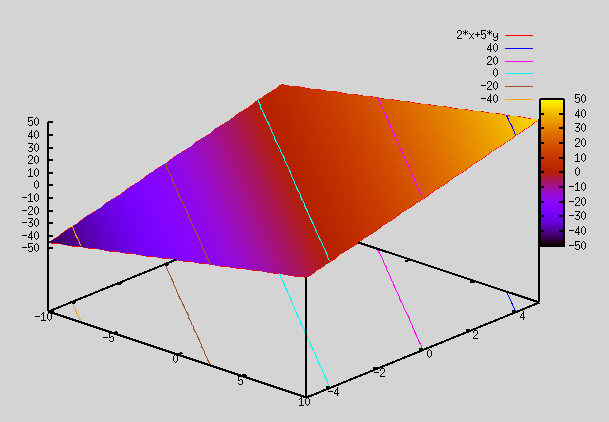
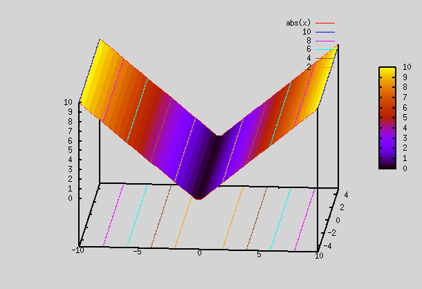
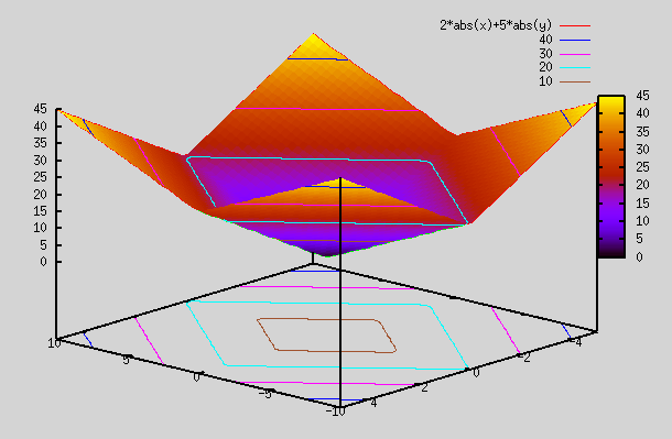
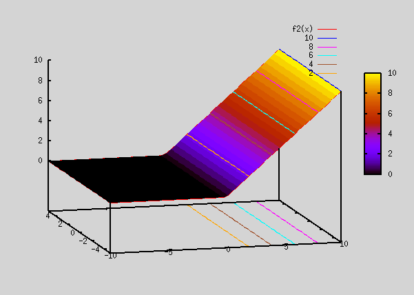
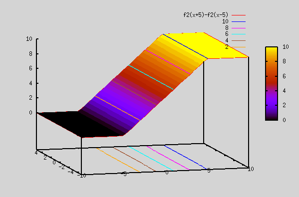
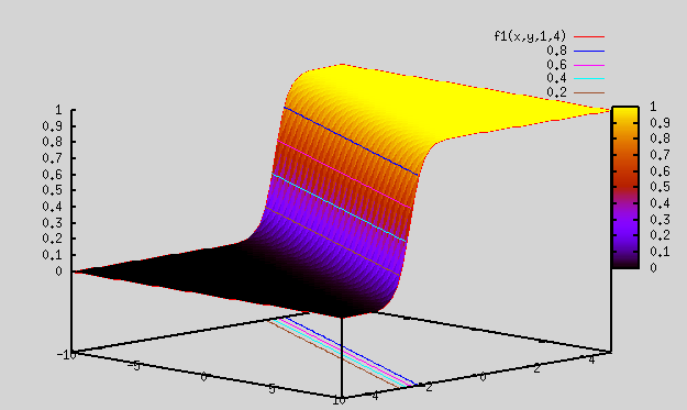
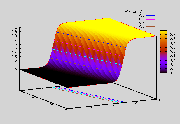
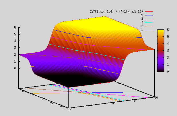
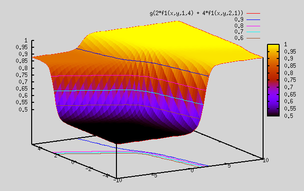
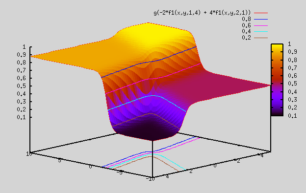
Let's revisit the section on "Best Fit Function". There we saw that sigmoid functions can be linearly added and fed into a sigmoid function to generate complex shapes. We saw plots for 2 dimensional i/p (i.e x,y), but it can be generalized to any number of inputs. By using appr weights and adding sigmoid functions, we were able to generate complex shapes.

ReLU or any other non linear functions can also be used instead of sigmoid functions.

NOTE: One very thing to keep in mind is that weight W need to be initialized to random values, instead of being initialized to 0. The lecture explains why.

Programming Assignment 1: This is a simple 2 layer NN. It tries to predict if a given dot is red or blue given it's location coordinate (x,y). Since the shape is in form of a flower, the 1 layer NN with it's linear equation can never form a boundary that can separate out the blue and red petals (as linear eqn can't form complex surface). Only 2 layer NN and higher layers can form a complex surface that can separate out various regions. We'll run our pgm thru both 1 layer NN and 2 layer NN.

Here's the link to pgm assigment:

Planar_data_classification_with_onehidden_layer_v6c.html

This project has 3 python pgm, that we need to understand.

A. testCases_v2.py => There are bunch of testcases here to test your functions as you write them. In my pgm, I've them turned off.

testCases_v2.py

B. planar_utils.py => this is a pgm that defines couple of functions. 

planar_utils.py

These functions are:

  • load_planar_dataset(): This function builds coordinates x1,x2 and corrsesponding color y (red=0, blue=1). The array X=(x1,x2) and Y for all the points is returned back. So, no database is loaded here from any h5 file. It's built within the function.
  • load_extra_datasets(): This loads other optional datasets as blobs, circles, etc. These are on same style as petals, where a linera logistic regression can never achieve high enough accuracy.
  • plot_decision_boundary(): This plots the 2D contour of the boundary where the function changes value from 0 to 1 or vice versa. However, this boundary is better visualized in 3D. So, I added options for 3D contour, 3D surface and 3D wireframe (on top of default 2D contour). I've set 3D surface as default, as that gives the best visual representation.
  • sigmoid(): This calculates sigmoid for a given x (x can be scalar or an array)

We'll import this file in our main pgm.

C. test_cr1_wk3.py => This pgm calls functions in planar_utils.  Here, we define our algorithm for 2 layer NN to find optimal weights, by trying out algorithm on training data.. We then apply those weights on training data itself to predict whether the whether the dots were red or blue. There is no separate testing data. We just want to see how well our surface fits training data. Below is the whole pgm:

test_cr1_wk3.py

Below are the functions defined in our pgm:

  • layer_sizes() => Given X,Y as i/p array, it returns size of input layer, hidden layer and output layer
  • initialize_parameters() => initializes W1,b1 and W2,b2 arrays. W1, W2 are init with random values (Very important to have random values instead of 0), while b1,b2 are init to 0. It puts these 4 arrays in dictionary "parameters" and returns that. NOTE: To be succinct, we will use w,b to mean W1,b1,W2,b2, going forward.
  • forward_propagation() => It computes output Y hat (i.e output A2). Given X, parameters (parameters has all w,b), this func calculates Z1, A1, Z2, A2 which are stored in dictionary "cache" and returned. NOTE: here didn't use sigmoid func for both layers. Instead we used tanh function for 1st layer (hidden layer), and sigmoid for next layer (output layer). Lectures explain it why.
  • compute_cost() => computes cost (which is the log function of A2,Y).
  • backward_propagation() => This computes gradients dw1, db1, dw2, db2 by using the formulas in lecture. It stores dw1, db1, dw2, db2 in dictionary "grads". It returns dictionary "grads". NOTE: above 3 functions were combined into one as propagate() in the previous exercise from week2, but here they are separated out for clarity.
  • update_parameters() => This function computes new w,b given old w,b and dw,db. It doesn't iterate here, rather iteration is done in nn_model() below
  • nn_model() => This is the main func that will be called in our pgm. We provide the training data array (both X,Y) as i/p to this func. It then returns to us the optimal parameters (w,b). It calls above functions as shown below:
    • calls func initialize_parameters() to init w,b,
    • It then iterates thru cost function to find optimal values of w,b that gives the lowest cost. It forms a "for" loop for predetermined number of iterations. Within each loop, it calls these functions:
      • forward_propagation() => Given values of X,w,b, it computes A2(i.e Y hat). It returns A2 and cache.
      • compute_cost() => Given A2,Y, parameters (w,b), it computes cost
      • backward_propagation => Given X,Y, parameters (w,b) and cache (which stores intermediate Z and A), it computes dw,db and stores it in grads.
      • update_parameters() => This computes new values of w,b using old w,b and gradients dw,db. New "parameters" dictionary is returned.
    • In beginning, w and b are initialized. We start the loop and in first iteration, we run the 4 functions listed above to get new w,b based on dw, db, and learning rate chosen. Then we start with next iteration. In next iteration, we repeat the process with newly computed values of w,b fed into the 4 functions to get even newer dw, db, and update w,b. We keep on repeating this process for "num_iterations", until we get optimal w,b which hopefully give lot lower cost than what we started with.
    • It then returns dictionary "parameters" containing optimal W1,b1,W2,b2
  • predict() => Given input picture array X and weight w,b, it predicts Y (i.e whether point is blue or not). It uses w,b calculated using nn_model() function. It calls forward_propagation() func to get A2 (i.e Y hat). If A2>0.5, it sets predictions to "1" else sets it to 0, and returns array "predictions".
  • Accuracy is then reported for all coordinates on what color they actually were vs what our pgm predicted.

Below is the explanation of main code (after we have defined our functions as above):

  1. We get our datset X,Y from any of the multiple sets available. We have our petal flower set (which is the default set). We can also choose optional noisy_circles, noisy_moons, blobs, gaussian_quantiles. We use func loadplanar_dataset() to load petal dataset, while we use load_extra_datasets() to load the other 4 datasets. We plot the data X,Y in a scatter plot. 
  2. We then run 2 classifiers on our data: 1 is logistic regression, while other is 2 layer NN:
    1. Logistic regression:
      1. Here we run logistic regression classifier on this X,Y dataset. Instead of building our own logistic regression classifier (as we did in week 2 exercise), we use sklearn's inbuilt classifier on X,Y set.
      2. We then use func plot_decision_boundary() to plot 2D/3D decision boundary (or predicted Y values, i.e Y hat values) to check how how fitting surface looks like with logistic regression classifier. It's a a single sigmoid function as expected (with a straight line seen in 2D contour)
      3. Then we print accuracy of logistic regression which is pretty low as expected.
    2. Two layer NN:
      1. Here we run our 2 layer NN. We call function nn_model() with i/p X,Y and number of hidden layers set to 4.
      2. Next, we use func plot_decision_boundary() to plot 2D/3D decision boundary (the same way as in regression classifier)
      3. Then we print accuracy of NN which is lot higher than logistic regression.
  3. In above exercise, we used a fixed number "4" for our hidden layer number. We would like to explore what does increasing the number of hidden layers do on the accuracy of prediction. So, we repeat the same exercise as we did in 2 layer NN, but now we vary hidden layer size from 1 to 50. As expected, larger the number of hidden layers, more the number of surfaces we have to play with, and hence better the fit we can achieve. So, prediction accuracy goes to 90%.

Below are the plots for different hidden layer size (sizes ranging from 1 to 20). NOTE: number of layers is still 2.

1. Petal data: First we show plots for Petal data set

A. below is how petal data looks like. Here o/p Y is the color, while i/p X are the coordinates (x1,x2)


B. When we run logistic regression on above data to get best fit, this is how logistic regression final output Y plot looks like:


C. Now, we run the same datset on optimal w,b calculated in our pgm above, but with different size of hidden layer ranging from 1 to 20. Here we plot A2 (not Y, but Y hat), so that we can see what values these sigmoid plots range from (i.e did they all the way to 0 or 1, or were they stuck in between values). If we plot finally Y (predicted values), then we lose this info. As can be seen, we get more and more tanh plots to arrange and get better fit, as we increase hidden layer size. Hidden layer size of 1 means only 1 tanh function, size=2 means 2 tanh functions, size=3 means 3 tanh functions, and so on. So, for size=3, activation function A2=C1*tanh+C2*tanh+C3*tanh can generate a lot more surfaces (about 3+3+1=7 possible surfaces).


2. noisy circles data: Next we show data for Noisy circles data set

A. below is how noisy circles data looks like. Here o/p Y is the color, while i/p X are the coordinates (x1,x2).

B. When we run logistic regression on above data to get best fit, this is how logistic regression final output Y plot looks like:


C. Now, we run the same datset on optimal w,b calculated in our pgm above, but with different size of hidden layer ranging from 1 to 20. As in petals case, we plot A2 (not Y, but Y hat). Results show the same thing as petals case: we get better fit, as we increase hidden layer size. Here blue and red dots are more randomly spread, so there should be more of  tanh functions that are added together, so that they can separate out red and blue dots. So, a larger hidden layer size helps.


Summary:

By finishing this exercise, we learnt how to build 2 Layer NN and figure out optimal weight for coordiantes (x,y) so that it can predict blue vs red dot. We played around with different size of hidden layer, and saw that higher the size of hidden layer, better is the fit, though beyond a certain optimal number, increasing the size of hidden layers don't add any extra value. We compared results to those predicted by logistic regression. Logistic regression (which is basically a single layer NN) could never match the accuracy provided by NN with 2 layer.

Course 1 - week 2 - Neural Network Basics:

This is the first technical introduction to NN. Well, the material for this week doesn't really talk about NN, it talks about regression, and how to do a linear and logistic regression. But in later weeks, you will see that these regressions are the simplest kind of NN. Logistic regression is a concept from statistics, but this defines the building block for AI.

For Linear and Logistic regression, see the AI section on "Statistics - Regression". This is all this week's lecture is about. Trying to do binary classification on a picture with nx pixels, to find out if it's a cat or not. First, we give m such training pictures to our regression engine, let it find weights which gives it the lowest cost, and then use the weights to predict on a test picture. If our weights are optimal, and the test picture is close to our training set picture, then our regression algo would do a good job in classifying the picture correctly.

However, just from common sense it looks like this approach of simple regression will never work, as cats can come in any color, shape, position, background, etc. Regression is just matching pixels and trying to minimize distance, it has no spatial information (i.e if there are 10 pixels next to each other to form a eye, then our logistic regression model doesn't care if these 10 pixels are on 10 different corners of the picture, or they are next to each other).

As an example, consider 8X8 pixel black and white picture. Each pixel can have 2 values: 0 for black and 1 for white. So, total possibilities of all pictures possible is 2^(8*8)=2^64 unique pictures possible. Our regression analysis is trying to go thru limited set of such possible combinations and predict what each picture is going to be. It's impossible to do that even for 8x8 pixel black and white picture. Just imagine how to do that for 64x64 colored picture !! And then for even larger pictures. It's just not possible by brute force "least error" regression technique. Something better has to be done. That's for later courses !!

 This week has a programming assignment, that is an absolute must to be completed, if you want to learn AI. It helps you go thru simplest NN that's possible, which is actually logistic regression. All new concepts are developed. Take your time to finish this assignment.

Programming Assignment 1: This is a simple image recognition pgm. It reads a file of images to get trained (using whatever algorithm we use, here we use logistc regression), and then we run the pgm on test images to see how well our algorithm works.

Here's the link to pgm assigment:

Logistic_Regression_with_a_Neural_Network_mindset_v6a.html

This project has 2 python pgm, that we need to understand.

A. lr_utils.py => this is a pgm that defines a function "load_dataset". We'll import this file in our main pgm. However, instead of writing it as a separate pgm, I copied the function defined in this file in the main python pgm.

The function load_dataset() reads 2 files: test data and training data. Below are the two h5 files that contain our training data and test data. Feel free to download the 2 files by right clicking and choosing "save link as" (If you directly click on the link below, it will open the h5 file in the browser itself, which will look garbage as it's not a text file that browser knows how to display):

train_catvnoncat.h5

test_catvnoncat.h5

1. training data: This data is used to train our algo. It has 209 training data set with label="train_set_x". It has 209 2D pictures, which are each 64x64 pixels, and each picture has a triplet of R,G,B values

2. testing dat: This data is used to test our algo. It has 50 testing data set with label="test_set_x". It has 50 2D pictures, which are each 64x64 pixels, and each picture has a triplet of R,G,B values.

 Below I'm writing the function "load_dataset" from lr_utils.py

import numpy as np
import h5py
    
def load_dataset():
    train_dataset = h5py.File('datasets/train_catvnoncat.h5', "r")
    train_set_x_orig = np.array(train_dataset["train_set_x"][:]) # your train set features. We store this data into an array of 209X64X64X3
    train_set_y_orig = np.array(train_dataset["train_set_y"][:]) # your train set labels. This stores the type=0 for non cat and 1 for cat corresponding to 209 pictures.It's a 1D array with 209 elements, but since it's 1D, we convert it to 2D array as shown later

    test_dataset = h5py.File('datasets/test_catvnoncat.h5', "r")
    test_set_x_orig = np.array(test_dataset["test_set_x"][:]) # your test set features. Similarly for test set, we have 50 pictures, array is 50X64X64X3
    test_set_y_orig = np.array(test_dataset["test_set_y"][:]) # your test set labels. This stores the type for these 50 pictures

    classes = np.array(test_dataset["list_classes"][:]) # the list of classes

    print("train = ",train_dataset, "test = ",test_dataset, "classes = ",classes,classes.shape)

    print("OLD", train_set_x_orig.shape, train_set_y_orig.shape, test_set_x_orig.shape, test_set_y_orig.shape)
    train_set_y_orig = train_set_y_orig.reshape((1, train_set_y_orig.shape[0]))
    test_set_y_orig = test_set_y_orig.reshape((1, test_set_y_orig.shape[0]))
    print("NEW", train_set_x_orig.shape, train_set_y_orig.shape, test_set_x_orig.shape, test_set_y_orig.shape)
    return train_set_x_orig, train_set_y_orig, test_set_x_orig, test_set_y_orig, classes


result:

train =  <HDF5 file "train_catvnoncat.h5" (mode r)> test =  <HDF5 file "test_catvnoncat.h5" (mode r)> classes =  [b'non-cat' b'cat'] (2,) => train_dataset, test_dataset are just pointers. classes is a 1D array with just 2 string values [non-cat cat]

OLD (209, 64, 64, 3) (209,) (50, 64, 64, 3) (50,) => The y labels are 1D array here
NEW (209, 64, 64, 3) (1, 209) (50, 64, 64, 3) (1, 50) => They y labels have been converted into 2D array here (X labels are still 4D array)


B. test_cr1_wk2.py => This pgm calls func load_dataset() defined in lr_utils, and we define our algorithm for logistic regression here to find optimal weights, by trying out algorithm on training data.. We then apply those weights on test data to predict whether the picture has a cat or not.

Below is the whole pgm, including the function defined in lr_utils.py

test_cr1_wk2.py

Below are the functions defined in our pgm:

  • sigmoid() => defines sigmoid func for any input z
  • initialize_with_zeros() => initializes w,b arrays with 0
  • propagate() => computes total cost. Given X, w, b, this func calculates activation A (which is the sigmoid function of linear eqn w1*x1+... wn*xn +b) and then computes cost (which is the log function of A,Y). Then it computes gradients dw, db. It stores dw, db in dictionary "grads". It returns scalar "cost" and dictionary "grads"
  • optimize() => This function iterates thru cost function to find optimal values of w,b that gives the lowest cost. It forms a "for" loop for predetermined number of iterations. Within each loop, it calls function propagate() with given values of X,w,b. In beginning, w and b are 0. propagate() returns new dw,db. Then it updates w,b with new values based on dw, db, and learning arte chosen. Then it starts with next iteration. In next iteration, it feeds newly computed values of w,b into propagate() to get even newer dw, db, and updates w,b. It keeps on repeating this process for "num_iterations", until it gets to w,b which hopefully give lot lower cost than what we started with.
  • predict() => Given input picture array X, it predicts Y (i.e whether pic is cat or not). It uses w,b calculated using optimize function. We can provide a set of "n" pictures here in single array X (we don't need to provide each pic individually as an array). This is done for efficiency purpose, as Prof Andrew explains multiple times in his courses.
  • model() => This is the main func that will be called in our pgm. We provide both training and test pictures as 2 big arrays as i/p to this func. It calls above functions as shown below:
    • calls func initialize_with_zeros() to init w,b,
    • then calls optimize() to optimize w,b to give lowest cost across the training set.
    • It then calls predict() to predict on any picture. predict is called twice for both training set and test set to predict cat vs non cat.
    • Accuracy is then reported for all pictures on what they actually were vs what our pgm predicted.

Below is the explanation of main code (after we have defined our functions as above):

  1. We load the datset X,Y for m pictures stored in h5 files.
  2. Then we enter in a loop, where we can repeat running this program as many times as we want for whatever reason. NOT really needed.
  3. Inside the loop, we flatten and normalize array X that we read from dataset in h5 file. We flaltten array of R,G,B pixels for each picture into shape(nx*nx*3,1). This flattening is done since our weight array also flattened. We want one weight for each pixel, so both weight and pixel value have to be 1D array, so that we can just multiply them directly as w1*x+w2*x2+...+wn*xn. In our implementation of this in numpy, we make them 2D array, but they still have only 1 row or col filled (i.e they behave like 1D).
  4. Now we run function model() on array X (which already has m training pics in it), and find optimal w,b by running it on training set. Function model() then runs prediction() and reports prediction accuracy for both training and test set.
  5. Then we have a choice of trying various learning rates, and see the effect on minimal cost achieved by our pgm. Learning rates matter a lot, as we see by trying small/large rates.
  6. Then finally we have a choice of trying 10 diff random images (these images are in all_data dir), which are predicted by calling predict(). Prediction value for each image is reported. We see that accuracy is bad (about 50%). Here we used Image module from PIL library. I couldn't get "imread" from matplotlib to work.

Summary:

By finishing this exercise, we learnt how to do logistic regression to figure out optimal weight for each pixel of a picture so that it can predict a cat vs non cat picture.


Intro to Deep Learning: Course 1 - Week 1

This is very introductory material.

Neural Network (NN) is just taking a dataset and fitting it with a eqn i.e given input features X1, X2, ... Xn, and a output Y, which we try to fit with a complex eqn Y = F(X1,X2,...,Xn). Once we find this best fit eqn F, we use this to predict Y given X1,X2,...Xn.

Process of getting this eqn is called network training. The term neural network came into being, since this complex eqn that we get resembles a chain of neurons passing information from one to the next, until we get to the output stage. From statistics, we know how to find best fit, but those eqn are flat (i.e Y=A*X+b*X^2+C*X^3...,). However, they never worked well on fitting new data, but these neural network based fitting eqn work well on new data too. They are very good with unstructured data (i.e identifying cat from a picture), while conventional fitting algorithms were good with only structured data (i.e predicting price of a house based on age, size, location, etc).

Diff kind of NN:

1. Standard NN

2. Convolutional NN

3. Recurrent NN

Deep Learning (DL): NN are called deep when they have a lot of layers. Reason, DL is getting so popular is because they work amazingly well. Reason for them working so well is due to the fact that deep neural network keep improving their prediction accuracy with more and more data, while earlier methodologies saturated and their prediction accuracy didn't improve even if they were loaded with more data.

 DL is very compute intensive since it needs to run thru large number of layers on lots of data.


Linear Functions:

Before we look into best fit functions, let's look at linear functions. Linear functions are functions that  satisfy these 2 requirements:

1. f(a*x) = a*f(x)

2. f(x+y) = f(x) + f(y)

These 2 requirements can be combined into one as f(a*x+b*y) = a*f(x)+b*f(y)

Linear functions are important as they state that any scaling and summation of linear functions is also linear and can be computed easily be separating the terms out. The single order polynomial f(x)=m*x+b is a linear function, while polynomials of higher order as f(x) = a*x^2 + b*x + c aren't.  But not all functions which look like linear are linear. We'll see examples below.

Best Fit Functions:

AI is all about finding a best fit function for any set of data. We saw in earlier article that for Logistic Regression, sigmoid sunction is a good function for best fit. However there is nothing special about a sigmoid function. From Fourier theorem, we know that a sum of sine/cosine functions can represent any function f(x) (with some limitations, but we'll ignore those). In fact, any function f(x) can be represented as infinite summation of polynomials of x (again with some limitations, but we'll ignore those). Sine/Cosine functions can also be represented as infinite summation of polynomials of x, so they are also able to represent any function f(x). Since any function can be rep as polynomial of x (Taylor's theorem), that implies that any function f(x) can be represented as summation of any other function g(x) that can be represented as infinite summation of polynomials. .

What about functions g(x) that are not infinite summation of x. Let's say g(x)=4+2*x. Will g(x) be able to represent any function f(x)? Since any func f(x) is infinite summation of polynomials, it can be approximated as finite sum of polynomials too. Of course, lower the number of polynomials terms we have in summation of f(x), less will be the accuracy in representing x. Let's see this with an example:

ex: f(x) = 3 + 7*x + 4*x^2 + 9*x^3 + .....

If g(x) = 4+2*x, then we can write f(x) = A*g(x). If we choose A=3, then then 3*g(x)=12+6*x, which is able to approximate f(x) though not exactly. Not only the higher powers of x are missing, but even the 1st 2 terms for f(x) don't match exactly with A*g(x). No matter how many linear combination of g(x) we use, we can't match the 1st 2 terms of f(x).

i.e f(x) = A1*g(x) + A2*g(x) = (A1+A2)*g(x), which is the same as B*g(x). So, we don't achieve anything better by summing the same function g(x) with different coefficients.

However, if we define 2 linear functions, g1(x) and g2(x), where g1(x)=4+2*x, while g2(x)=1+3*x, then A1*g1(x) + A2*g2(x) can be made to represent 3+7*x, by choosing A1=1/5, A2=11/5. Thus we are able to match 1st 2 terms of f(x) exactly.

However, if we had flexibility in choosing g(x), then we would choose g(x)=3+7*x. Then the 1st 2 terms of f(x) would match exactly with g(x), by using just 1 func g(x)

Similarly, if g(x) is chosen to be 2nd degree polynomial, i.e g(x)=1+2*x+3*x^2, then we can choose g1(x), g2(x), g3(x) to be 3 different 2nd degree poly eqn, and approximate f(x)=A1*g1(x) + A2*g2(x) + A3*g3(x). Or if we had flexibility in choosing g(x), then we would choose g(x)=3+7*x+4*x^2. Then the 1st 3 terms of f(x) would match exactly with g(x).

Continuing the same way, higher the order of g(x), closer will the approximation of f(x) with linear summation of any function g(x).

X as a multi dimensional vector:

Now let's consider eqn in n dimension, where f(x) is not a eqn in single var "x", but in "n" var x1,x2,...xn. i.e we define f(X) where X=(x1 x2 x3 .... xn).

Let's stick to 1st degree linear eqn g(x)=m*x+c. We define g1(x1)=m1*x1+c1, g2(x2)=m2*x2+c2, .... gn(xn)=mn*xn+cn

Then f(x1,x2,...,xn) = g1(x1)+g2(x2)+...+gn(xn) = m1*x1+c1 + m2*x2+c2 + .... mn*xn+cn = m1*x1 + m2*x2 + ... mn*xn + (c1 + c2 + ... + cn) = m1*x1 + m2*x2 + ... mn*xn + b (where b = c1+c2+...+cn)

So, for n dimensional space, if we choose g(x1,x2,...,xn) = m1*x1 + m2*x2 + ... mn*xn + b, then we can get a best fit n dimensional plane to function f(x1,x2,...,xn). However, the approximation function is 1st degree polynomial, so it doesn't have any curves or bends (just flat plane). This is a linear function.

Linear function with bendings:

What if we are able to introduce a bend in linear function g(x), so that it's not a straight line anymore. If we then add up these functions with bends, we can have any kind of bend desired at any point. Then we may be able to approximate any function f(x) with these function g(x) by having a lot of these g(x) functions with bends.

Let's see this in 3D, since multidimensional is difficult to visualize. We write above f(x) in 2D as:

f(x,y)=m1*x + m2*y = 2*x+5*y

gnuplot> splot 2*x+5*y => As seen below, this plot is a plane


Now, we take a simple function called absolute function. It has a bend, and slopes of 2 lines for x<0 and x>0 are -ve of each other.

gnuplot> splot abs(x) => As seen below, this plot has a bend at x=0


Now, we plot the same function as first one, but this time with abs functions applied to x and y. As you can see, we have bends so that we can generate planes at different angles to fit complex curves.

gnuplot> splot 2*abs(x)+5*abs(y)


 Is abs() function linear? It does look linear, but it has a bend (so 2 linear functions in 2 range).

Let's pick 2 points: x1=1 and x2=-1. Then abs(x1+x2) = abs(1-1) = abs(0) = 0. However, if we compute f(x1) and f(x2), we get f(-1)=1, and abs(1)=1. So. abs(x1)+abs(x2) = 2 which is not same as abs(x1+x2). So, abs() function is not linear. Similarly any 1st order eqn with a bend is not linear.

Taylor theorem tells us that any function can be expanded into infinite polynomial series. We should be able to find Taylor series for abs(x) function.

Note: f(x) = abs(x) = √(x^2) = √(1+(x^2 - 1)) = √(1+t) where t = (x^2 - 1)

√(1+t) is a binomial series which can be expanded into Taylor series as explained here: https://en.wikipedia.org/wiki/Binomial_series#Convergence

(1+t)^1/2 = 1 + (1/2)t - (1/(2*4))t^2 + ((1*3)/(2*4*6))t^3 - ...

So, f(x) = abs(x) = 1 + (x^2-1)/2 - (1/(2*4))(x^2-1)^2 + ((1*3)/(2*4*6))(x^2-1)^3 - ... = [1-1/2-1/(2*4)-...] + x^2*[1/2+1/4+...] + x^4*[-1/(2*4)+....] + x^6*[...] + ...

Thus we see that we get Taylor series expansion of abs(x) as summation of even powers of x. So, it is indeed not a linear eqn. As it's infinite summation, it can be used to represent any function as explained at top of this article.

ReLU function:

Just as absolute func has a bend and is not linear, many other linear looking functions can be formed which have a bend, but are not linear. One such function that is very popular in AI is ReLU (Rectified linear unit). Here instead of having slope as -1 for x<0, we make the slope=0 for x<0. This function is defined as below:

Relu(x) = x for x>0, = 0 for x<0

gnuplot> f2(x)=(x>0) ? x : 0 #this is the eqn to get a ReLu func in gnuplot
gnuplot> splot f2(x)

The above plot looks similar to how abs(x) function looked like, except that it's 0 for all x <0.

Now, let's plot a function which is a difference of the 2 Relu plots.

gnuplot> splot f2(x+5)-f2(x-5)

The Relu plot above ( Relu(x+5) - Relu(x-5) ) now has 2 knees at x=-5 and x=+5. It actually resembles a sigmoid function (explained below). However, it doesn't have smooth edges as in sigmoid func. Since sigmoid function can fit any func, linear sum of Relu func can also fit any func. The advantage with Relu is that it's similar to linear (it's linear in 2 separate regions, although it's not linear overall), so derivatives are straight forward.

There is very good link here on why Relu functions work so well in curve fitting (and how are they non-linear inspite of giving an impression of a linear eqn):

https://towardsdatascience.com/if-rectified-linear-units-are-linear-how-do-they-add-nonlinearity-40247d3e4792


Sigmoid function:

Sigmoid function being an exponential function, it's has higher powers of x in it's expansion, instead of just having "x" (i.e x, x^2, x^3, etc).

i.e σ(z) = 1 / (1 - e^(-z)) = A1 + A2*z + A3*z^2 + ... (taylor expansion)

Sigmoid function would fit better than Relu functions above as they have higher orders of x (so they have smooth edges). However, the are also more compute intensive, and so are not used except when absolutely necessary.

Let's plot a 2D sigmoid funcion, where z=a*x+b*y. We use gnuplot to plot the functions below:

 f1(x,y,a,b)=1/(1+exp(-(a*x+b*y)))

Plot 0:

gnuplot> splot f1(x,y,1,4) => As seen below, this is a smooth function varying from 0 to 1. Looks kind of similar to difference of Relu function plotted above.

Plot 1:

gnuplot> splot f1(x,y,2,1) => As seen below, plot is same as that above, except that the slope direction is different

Plot 2:

gnuplot> splot (2*f1(x,y,1,4) + 4*f1(x,y,2,1)) => Here we multiply the above 2 plots by different weights and add them up. So, resulting plot is no longer b/w 0 and 1, but varies from 0 to 6.


We define another sigmoid function, which is in 1 dimension

 g(x) = 1/(1+exp(-(x)))

Plot 3:

gnuplot> splot g(2*f1(x,y,1,4) + 4*f1(x,y,2,1)) => Here we took sigmoid of above plot, so resulting plot is confined to be b/w 0 and 1. However, because of the weights we chose, resulting plot ranges from 0.5 to 1, instead of ranging from 0 to 1.

Plot 4:

gnuplot> splot g(-2*f1(x,y,1,4) + 4*f1(x,y,2,1)) => almost same plot as above, except that z range here is from 0.1 to 1 (by changing weight to -ve number)


Summary:

 Now, that we know Relu and sigmoid functions are not linear, and in fact are polynomials of higher degree. As such, they can be used to represent any function, by using enough linear combinations of these functions. So, they can be used as fitting functions to fit any n dimensional function. These are used very frequently in AI to fit our training data. We will look at their implementation in AI section.

Course 1 - week 4 - Deep Neural Network:

This is week 4 of Course 1. Here we generalize NN from 1 hidden layer to any number of hidden layers. Maths get complicated, but it's repeating the same thing as in 2 Layer NN. 2 layer NN has one hidden layer and 1 output layer. L layer neural network has (L-1) hidden layers and 1 output layer. We don't count input layer in the number of layers.

There are few formulas here for forward and backward propagation. these form the backbone of DNN. These formula are summarized here:

https://www.coursera.org/learn/neural-networks-deep-learning/supplement/E79Uh/clarification-about-what-does-this-have-to-do-with-the-brain-video

There is very good derivation of all these equations here:

https://medium.com/@pdquant/all-the-backpropagation-derivatives-d5275f727f60

There are 2 programming assignments in this week: First we build a 2 layer NN and then a L layer NN to predict cat vs non-cat in given pictures. 2 Layer NN is just a repeat from last week's exercise, while L layer NN is generalization of 2 layer NN.

Programming Assignment 1: Here we build helper functions to help build a deep NN.  We also build helper function for a 2 layer NN separately.

Here's the link to pgm assigment:

Building_your_Deep_Neural_Network_Step_by_Step_v8a.html

This project has 3 python pgm, that we need to understand.

A. testCases_v4a.py => There are bunch of testcases here to test your functions as you write them. In my pgm, I've them turned on.

testCases_v4a.py

B. dnn_utils_v2.py => this is a pgm that defines couple of functions. 

dnn_utils_v2.py

These functions are:

  • sigmoid(): This calculates sigmoid for a given Z (Z can be scalar or an array). Output returned is both A (which is sigmoid of Z), and cache (which is same as i/p Z)
  • sigmoid_backward(): This calculates dZ given dA and Z. dZ = dA*σ(Z)*[1-σ(Z)]. We stored Z in cache (in sigmoid() above)
  • relu(): This calculates relu for a given Z (Z can be scalar or an array). Output returned is both A (which is relu of Z), and cache (which is same as i/p Z)
  • relu_backward(): This calculates dZ given dA and Z. dZ = dA for A>0 else dZ=0. We stored Z in cache (in relu() above)

We'll import this file in our main pgm.

C. test_cr1_wk4_ex1.py => This pgm just defines the helper functions that we'll call in our 2 layer and L layer NN model that we define in assignment 2. Below is the whole pgm:

test_cr1_wk4_ex1.py

Below are the functions defined in our pgm:

  • initialize_parameters() => This function exactly same as previous week's function for 2 Layer NN. Input to func is size of i/p layer, hidden layer and output layer. It initializes W1,b1 and W2,b2 arrays. W1, W2 are init with random values (Very important to have random values instead of 0), while b1,b2 are init to 0. It puts these 4 arrays in dictionary "parameters" and returns that. NOTE: To be succinct, we will use w,b to mean W1,b1,W2,b2, going forward.
  • initialize_parameters_deep() =>This initializes w,b for L layer NN (same as for 2 layer NN, but extended to L laeys). i/p is an array containing sizes of all the layers, while o/p is initialized W1,b1, W2, b2, .... WL,bL for L layer NN. All weights are bias are stored in dictionary "parameters"
  • Forward functions: These are functions for forward computation:
    • linear_forward() => It computes output Z, given i/p A, W, b. Z = np.dot(W,A)+b. this is calculated for a single layer, using i/p A (which is the o/p from previous layer) and computing Z. It returns Z and linear_cache which is a tuple containing (Aprev,W,b), where Aprev is for previous layer, while W, b are for current layer.
    • linear_activation_forward() => This computes activation A for Z that we calculated above for layer "l". The reason we separated out the 2 functions for computing Z and A, is because A requires 2 diff functions, sigmoid or relu for computing A (depending on which one we want to use for current layer. sigmoid is used for output layer, while relu is used for all other layers). This keeps code clean.
      • We call following functions:
        • linear_forward() => returns Z, linear_cache
        • sigmoid() => returns A, activation_cache
        • relu() => returns A, activation_cache
      • We store all relevant values in tuple cache:
        • linear_cache => stores tuple (Aprev,W,b), where Aprev is for previous layer, while W, b are for current layer.
        • activation_cache => stores computed Z for current layer
        • cache => stores tuple (linear_cache, activation_cache) = (Aprev, W, b, Z). In previous week example, we used cache to store A, Z for both layers (A1, Z1, A2, Z2), but here we store W, b too for each layer on top of A (for previous layer) and Z (for current layer) in tuple cache.
      • The function finally returns A for current layer and cache. So, we end up returning (Aprev, W, b, Z, A), where Aprev is for previous layer, while W, b, Z, A are for current layer.
    • L_model_forward() => This function does forward computation staring from i/p X, and generating o/p Y hat  (i.e output AL for last layer L). This is same as forward_propagation() function that we used in last week's example. It's just more complicated now, since it involves L layers now, instead of having just 2 layers. We define tuple "caches", which is just all cache appended.
      • From layer 1 to layer (L-1) (hidden layers), we call function linear_activation_forward()  with "Relu" function in a for loop (L-1) times
        • In each loop, cache and A are returned for that layer. A is used in next iteration, while cache is appened to tuple "caches"
      • For last layer L (o/p layer), we again call function linear_activation_forward(), but this time with "sigmoid" function
        • cache and AL are returned for last layer. AL is going to be used in compute_cost() function (defined below), while cache is appened to tuple "caches"
  • compute_cost() => computes cost (which is the log function of AL,Y).
  • Backward functions: These are functions for forward computation. They are the same as their forward conterpart, just going backward from layer L to layer 1.
    • linear_backward() => This is the backward counterpart of linear_forward() func. Given i/p cache and dZ for a given layer, it computes gradients dW, db, dA. Input cache stores tuple (Aprev, W, b). NOTE: dW computation requires A from previous layer
      •     A_prev, W, b = cache 
      •     dW = 1/m * np.dot(dZ,A_prev.T)
      •     db = 1/m * np.sum(dZ,axis=1,keepdims=True)
      •     dA_prev = np.dot(W.T,dZ)
    • linear_activation_backward() => This is the backward counterpart of linear_activation_forward() func. Instead of computing A from Z, this computes dA for previous layer given dA (from which dZ is computed) for current layer.
      • We call following functions (same as what used in linear_activation_forward(), but now in backward dirn):
        • sigmoid_backward() => returns dZ given dA for sigmoid func
        • relu_backward() => returns dZ given dA for relu func
        • linear_backward()=> using dZ returned by sigmoid/relu backward func above, it computes dA_prev, which is dA for previous layer (since we are going in reverse dirn)
      • The function finally returns dA for previous layer and dW, db for current layer.
    • L_model_backward() => This is the backward counterpart of L_model_forward(). This function does backward computation staring from o/p Y hat  (i.e output AL for last layer L) and going all the way to the input X. It returns dictionary "grads" containing dW, db, dA.
      • dAL = - (np.divide(Y, AL) - np.divide(1 - Y, 1 - AL))
      • dA{L-1}, dWL, dbL => computed using func linear_activation_backward() for layer L. Uses dAL from above as i/p to this func
      • Now, we run a loop from layer L-1 to layer 1 to compute dA, dW, db for each layer "l"
        • dA{l-1}, dWl, dbl => computed using func linear_activation_backward() for layer "l". Uses dAl from prev iteration as i/p to this func to compute dA{l-1}. It uses dA{L-1} from above for l=L-1 to compute da{L-2} and then keeps on iterating backward.
      • Finally it returns dictionar grads containing dW, db, dA for each layer
  • update_parameters() => This function is same as that in previous week exercise. computes new w,b given old w,b and dw,db, using the learning rate provided. This is done for w,b for all layers 1 to L (i.e W1=W1-learning_rate*dW1, b1=db1-learning_rate*dW1, .... , WL=WL-learning_rate*dWL, bL=dbL-learning_rate*dWL)
  • 2_layer_model()/L_layer_model => These are the main func, but they are not called here. They are part of assignment 2.


Programming Assignment 2: Here we use helper functions defined above in assignment 1 to help build a 2 Layer shallow NN and a L layer deep NN. We find optimal weights using training data and then apply those weights on test data to predict whether the picture has a cat or not.

Here's the link to pgm assigment:

Deep+Neural+Network+-+Application+v8.html

This project has 2 python pgm, that we need to understand.

A. dnn_app_utils_v3.py => this is a pgm that defines all the functions that we defined in assignment 1 above (both from dnn_utils_v2.py and test_cr1_wk4_ex1.py). So, either we can use our functions from assignment 1 or use functions in here. If you wrote all functions in assignment 1 correctly, then it should match all functions in this pgm below (except for few difference noted below).

dnn_app_utils_v3.py

The few differences to note in above pgm are:

  • load_data() function: This function is extra here. It is exactly same as load_dataset() that we used in week2 assignment to load cat vs no cat dataset. Here too we load the same cat vs no cat dataset that's in h5 file.
  • predict(): This prints accuracy for any i/p set X (which can have multiple pictures in it). It uses w,b and generates output y hat for the given X. If y hat > 0.5, it predicts it as cat, else non cat. It then compares the results to actual y values, and prints accuracy. It only calls 1 function=> L_model_forward. In returns probability array "p" for all pictures. I added extra var "probas" (which is the output value y hat), so that we can how close or far off were different predictions, even if they were correct or wrong. This gives us a sense of how our algorithm is doing.
  • print_mislabeled_images(): This takes as i/p dataset X,Y along with predicted Y hat, and plots all images that aren't same as what was predicted (i.e wrongly classified)
  • IMPORTANT: initialize_parameters_deep() function: This function is same as what we wrote in assignment 1 above, with a subtle difference. Here we use a different number to initialize w. Instead of multiplying the random number by 0.01, we multiply it by 1/ np.sqrt(layer_dims[l-1]) for a given layer l. As you will see, this causes a lot of difference in getting the cost low. With 0.01, our cost starts at 0.693148, and remains at 0.643985 at 2400 iteration. Accuracy for training data remains low at 0.65. However, using the new sqrt multiplier, our cost starts at 0.771749, and goes down to 0.092878 at iteration 2400, giving us a training data accuracy of 0.98.

We'll import this file in our main pgm below

B. test_cr1_wk4_ex2.py => This pgm calls functions in dnn_app_utils_v3.py.  Here, we define our algorithm for 2 layer NN and L layer NN by calling functions defined above. We find optimal weights, by trying out algorithm on training data.. We then apply those weights on test data to see how well our NN predicts cat vs non cat. Below is the whole pgm:

test_cr1_wk4_ex2.py

Below are the functions defined in our pgm:

  • two_layer_model() => This function implements a 2 layer NN. It is mostly same as previous week's function for 2 Layer NN which was called nn_model(). The big difference is that we used tanh() function for hidden layer, while here we'll use relu function for hidden layer. Input to func is size of i/p layer, hidden layer and output layer. On top of that we provide i/p dataset X, o/p dataset Y and a learning rate. The function returns optimal W1,b1,W2,b2., These are the steps in this function:
    • calls func initialize_parameters() to init w,b
    • It then iterates thru cost function to find optimal values of w,b that gives the lowest cost. It forms a "for" loop for predetermined number of iterations. Within each loop, it calls these functions:
      • linear_activation_forward() => Given values of X,W1,b1, it calls func linear_activation_forward()  with relu to get A1. It then calls linear_activation_forward()  again with A1,W2,b2 and sigmoid to get A2. computes A2(i.e Y hat). It returns A2 and cache.
      • compute_cost() => Given A2,Y,  it computes cost
      • Then it calc initial back propagation for dA2 = - (np.divide(Y, A2) - np.divide(1 - Y, 1 - A2))
      • linear_activation_backward => Given dA2 and cache, it calls linear_activation_backward to get dA1, dW2, db2. It then calls linear_activation_backward()  again with dA1 and cache to get dA0, dW1,db1. It stores dW1,db1,dW2,db2 in dictionary grads.
      • update_parameters() => This computes new values of parameters using old parameters and gradients from grads.
    • In beginning, w and b are initialized. We start the loop and in first iteration, we run the 4 functions listed above to get new w,b based on dw, db, and learning rate chosen. Then we start with next iteration. In next iteration, we repeat the process with newly computed values of w,b fed into the 4 functions to get even newer dw, db, and update w,b. We keep on repeating this process for "num_iterations", until we get optimal w,b which hopefully give lot lower cost than what we started with.
    • It then returns dictionary "parameters" containing optimal W1,b1,W2,b2
  • L_layer_model() => This function implements a L layer NN. It's just an extension of 2 layer NN. Input to func is size of i/p layer, hidden layer and output layer. On top of that we provide i/p dataset X, o/p dataset Y and a learning rate. The function returns optimal W1,b1,...,WL,bL., These are the steps in this function:
    • calls func initialize_parameters_deep() to init w,b
    • It then iterates thru cost function to find optimal values of w,b that gives the lowest cost. It forms a "for" loop for predetermined number of iterations. Within each loop, it calls these functions:
      • L_model_forward() => Given values of X,W1,b1, it calls func linear_activation_forward()  with relu to get A1. It then calls linear_activation_forward()  again with A1,W2,b2 and sigmoid to get A2. computes A2(i.e Y hat). It returns A2 and cache.
      • compute_cost() => Given A2,Y,  it computes cost
      • Then it calc initial back propagation for dA2 = - (np.divide(Y, A2) - np.divide(1 - Y, 1 - A2))
      • L_model_backward => Given dA2 and cache, it calls linear_activation_backward to get dA1, dW2, db2. It then calls linear_activation_backward()  again with dA1 and cache to get dA0, dW1,db1. It stores dW1,db1,dW2,db2 in dictionary grads.
      • update_parameters() => This computes new values of parameters using old parameters and gradients from grads.
    • In beginning, w and b are initialized. We start the loop and in first iteration, we run the 4 functions listed above to get new w,b based on dw, db, and learning rate chosen. Then we start with next iteration. In next iteration, we repeat the process with newly computed values of w,b fed into the 4 functions to get even newer dw, db, and update w,b. We keep on repeating this process for "num_iterations", until we get optimal w,b which hopefully give lot lower cost than what we started with.
    • It then returns dictionary "parameters" containing optimal W1,b1,...,WL,bL

Below is the explanation of main code (after we have defined our functions as above):

  1. We load our datset X,Y by using func load_data(). We then flatten X and normalize X (by dividing it by 255)
  2. We then run 2 NN on our data: 1 is 2 layer NN, while other is L layer NN. We can choose which one to run by setting appr variable. Size of i/p layer for both examples below is fixed to 12288 (64*64*3 which is the total number of data points associated with 1 picture). Size of o/p layer is fixed to 1 (since our o/p contains just 1 entry: 0 or 1 for cat vs non cat). Size of hidden layers is what we can play with, since it can be varied to any number we want.
    1. 2 layer NN:
      1. We call two_layer_model()  on this X,Y training dataset. We give dim of i/p layer, hidden layer and output layer, and set num of iterations to 2500. Hidden layer size is set to 7.
      2. Then we call  predict() to print accuracy on both training data and test data which is pretty low as expected.
      3. Then we print mislabeled images by calling func print_mislabeled_images.
    2. L layer NN:
      1. We call function L_layer_model() with i/p X,Y training dataset and number of hidden layers set to 3 (So, it's a 4 layer NN).
      2. Then we call  predict() to print accuracy of L NN on both training data and test data,  which is lot higher than 2 layer NN.
      3. Then we print mislabeled images by calling func print_mislabeled_images.
  3. Then we run the NN (2 Layer or L layer depending on which one is chosen) on our 10 picture dataset that I downloaded from internet (same as what we used in lecture 1, week 2 example). These are all cat pictures. In predict(), we return "y hat" also, so we are able to see all predicted values.

Results:

On running above pgm, we see these results:

2 layer NN: It achieves 99.9% accuracy on training data, but only 72% on test data.

 Cost after iteration 0: 0.693049735659989

...

Cost after iteration 2400: 0.048554785628770226
Accuracy: 0.9999999999999998
Accuracy: 0.72

When I run it thru my 10 random cat pictures downloaded from internet, I get 90% accuracy. Below are the A (y hat) value and the final predicted value . As can be seen, accuracy is very low at 60%.  Even for ones that were predicted correctly, y hat activation values are not 99% for all correct ones.

Accuracy: 0.6
prediction A [[0.2258492  0.88753723 0.04103057 0.97642935 0.87401607 0.85904489 0.49342905 0.99138362 0.96587573 0.3834667 ]]
prediction Y [[0. 1. 0. 1. 1. 1. 0. 1. 1. 0.]]

4 layer NN: It achieves 99% accuracy on training data and 80% accuracy on test data. For 1st layer, size=20, 2nd layer size=7, 3rd layer size=5 and 4th layer size=1 (since it's o/p layer). size of i/p layer is 12288.

Cost after iteration 0: 0.771749

.........

Cost after iteration 2400: 0.092878
Accuracy: 0.9856459330143539
Accuracy: 0.8

 As in 2 Layer NN, when we run 4 layer NN thru the same 10 random cat pictures, I get 90% accuracy which is lot higher than 2 layer NN. Below are the A (y hat) value and the final predicted value . As can be seen, even though accuracy is 90%, the algorthm completely failed for picture 10 which is reported as 0.2, even though it's a perfect cat picture (may be the background color made all the difference. Will need to check it with different background color to see if it makes any difference). The other picture that is right on borderline is the 6th picture. Here, may be too much background noise (things around the cat) is causing the issue. Will need to check with different background to see if that helps.

Accuracy: 0.9

prediction A [[0.99930858 0.97634997 0.96640157 0.9999905  0.95379876 0.5026841 0.92857836 0.99693246 0.99285584 0.21739979]]
prediction Y [[1. 1. 1. 1. 1. 1. 1. 1. 1. 0.]]

Initialization of w,b: If we used the initialization multiplying factor of 0.01 instead of 1 / np.sqrt(layer_dims[l-1]), we'll get a very bad accuracy: 65% on training set and 34% on test set. even worse is the fact that on our 10 random cat images, we get 0% accuracy. This all with just using a different initialization number for different layers. Perhaps this will be explored in next lecture series.

This is what initialization multiplying factor is for different layers (instead of using constant 0.01 for all layers, we increase this value as size of layer increases):

l= 1 => 1 / np.sqrt(layer_dims[l-1]) = 1 / np.sqrt(12288) = 0.009

l=2 => 1 / np.sqrt(layer_dims[l-1]) = 1 / np.sqrt(20) = 0.22

l=3 => 1 / np.sqrt(layer_dims[l-1]) = 1 / np.sqrt(7) = 0.38

l=4 => 1 / np.sqrt(layer_dims[l-1]) = 1 / np.sqrt(5) = 0.45

NOTE: Do NOT forget to change this multiplying factor of 0.01 if you plan to use your own functions from assignment 1 above.

Summary:

Here we build a 2 layer NN (with 1 hidden layer) as well as a L layer NN (with L-1 hidden layers). We can play around with lot of parameters here to see if our L layer NN (here we chose L=4) performs better with more layers, or more hidden units in each layer, or with a different initialized values, or different learning rates, etc. It's hard to say which of these values will give us the optimal results without trying it out. This will be the topic for Course 2 series.