Probability Distribution

We looked at pdf (probability distribution function) earlier. A probability distribution can either be univariate or multivariate

  1. Univariate: A univariate distribution gives the probabilities of a single random var taking on various alternative values;
  2. Multivariate: A multivariate distribution gives the probabilities of a random vector—a set of two or more random variables—taking on various combinations of values. 

Normal Distribution:

There are many kinds of univariate/multivariate distribution function, but we'll mostly talk about "Normal Distribution" aka "Guassian distribution" (or bell shape distribution). Normal distribution is what you will encounter in almost all practical examples in semiconductors, AI, etc. So makes sense to study normal dist in detail. Yu can read about many other kind of dist in wikipedia link:

1. Univariate normal distribution:

https://en.wikipedia.org/wiki/Normal_distribution

pdf function is:

f(x) = 1/(σ√2π).exp(-1/2*((x-μ)/σ)2) => Here μ=mean, σ=std deviation (or σ2= variance). We divide it by σ, so that the integral of f(x) is 1.

Standard normal distribution is simplest normal dist with μ=0, σ=0.

The way we write that random var X belongs to normal distrbution is via this notation:

X ~ N(μ, σ2) => Here N means normal distribution. mean and variance are provided.

We often hear 1σ, 2σ, terms. These refer to σ in Normal dist. If we draw pdf for normal distribution and try to calculate as to how many samples lie within +/- 1σ, we see that 68% of the values are within 1σ or 1 std deviation. Similarly fo 2σ, it's 95%, while for 3σ, it's 99.7%. 3σ is often referred to as 1 out of 1000 outside the range. So that implies that 3σ is roughly taken as 99.9% even though it's 99.7% when solved.

As 3σ is taken as 1 out of 103 or 10-3, 4σ is taken as 10-4, 5σ as 10-5 and 6σ as 10-6 event. So, 6σ implies only 1 out of 1M chance of the sample ebing outside the range. 6σ is used very commonly in industries. Many products have requirement of 6σ defects, i.e 1 ppm defect (only 1 out of 1M parts is allowed to be defective). In semiconductors, 3σ defect rate is targeted for a lot of parameters.


2. Multivariate normal distribution: It's generalization of one dimenesional univariate normal dist to higher dimensions.

 https://en.wikipedia.org/wiki/Multivariate_normal_distribution

A random vector X = X1,X2,...Xn is said to be multivariate normal dist if Every linear combination {\displaystyle Y=a_{1}X_{1}+\cdots +a_{k}X_{k}} of its components is normally distributed.

A Multivariate Normal dist is hard to visualize, and not that common. A more common case of multivariate normal dist is bivariate normal dist which is normal dist with dimension=2.

Bivariate normal distribution: Given 2 random vector X, Y, a bivariate pdf function is:

f(x,y) = 1/(2πσx σy √(1-ρ2)).exp(-1/(2(1-ρ2))*[ ((x-μx)/σx) - 2ρ(x-μx)/σx*(y-μy)/σy +  ((y-μy)/σy)2 ]  => Here μ=mean, σ=std deviation (or σ2= variance). We defined a new term rho (ρ), which is the Pearson correlation coefficient R b/w X and Y. It's the same Pearson coeff that we saw earlier in stats section. rho (ρ) captures the dependence of Y on X. If Y is independent of X, then ρ=0, while if Y is completely dependent on X, then ρ=1. We will see more examples of this later. We divide this expr by complex looking term, so that the 2D integral of f(x,y) is 1.

2D plot of f(x,y): We will use gnuplot to plot these.

This is the gnuplot pgm (look in gnuplot section for cmds and usage). f_bi is the final func for Bivariate normal dist func.

gnuplot> set pm3d
gnuplot> set contour both
gnuplot> set isosamples 100
gnuplot> set xrange[-1:1]
gnuplot> set yrange[-1:1]
gnuplot> f1(x,y,mux,muy,sigx,sigy,rho)=((x-mux)/sigx)**2 - 2*rho*((x-mux)/sigx)*((y-muy)/sigy) + ((y-muy)/sigy)**2
gnuplot> f_bi(x,y,mux,muy,sigx,sigy,rho)=1/(2*pi*sigx*sigy*(1-rho**2)**0.5)*exp((-1/(2*(1 - rho**2)))*f1(x,y,mux,muy,sigx,sigy,rho))

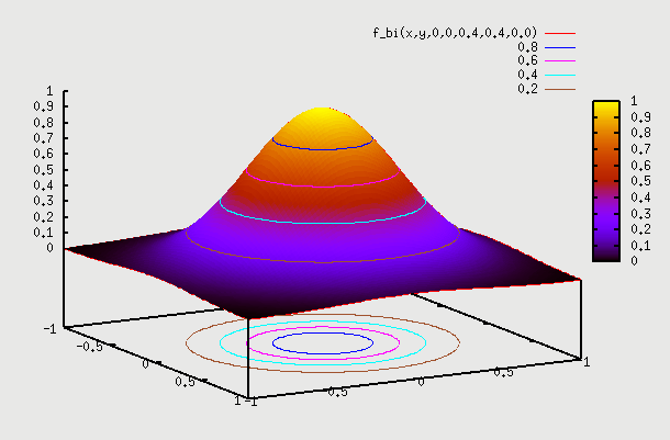
1. f(x,y) with ρ=0 => Let's say we have sample of people where X is their height and Y is their IQ. We don't expect to have any dependence between the two. So, here f(X) on X axis is the height of people which is a 1D normal distribution around some mean. Similarly f(Y) on Y axis is the IQ of people which is again a 1D normal distribution around some mean. If we plot a 2D pdf of this, then we are basically multiplying probability of X with probability of Y to get probability at point (x,y). Superimposing f(X) and f(Y) gives contour as a circle as X=mean+sigma or X=mean-sigma will yield the same value for Y as probability of Y doesn't change based on what the probability of X is. Infact this is the properrty and definition of independence => if f(x,y)=f(x).f(y) that means X and Y are independent. We can see that setting ρ=0 yields that. Below is the gnuplot function and the plot

gnuplot> splot f_bi(x,y,0,0,0.4,0.4,0.0)

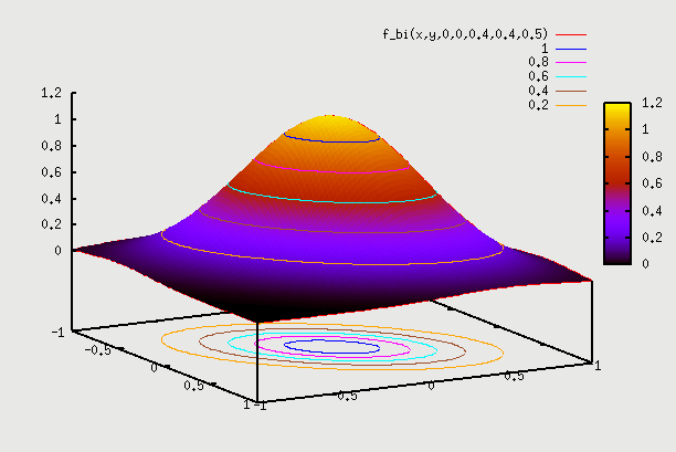
2. f(x,y) with ρ=0.5 =>Here we can consider the example of same people as above but plot weight Y vs Height X. We hope to see some correlation. What this means is that pdf(Y) varies depending on which point X is chosen. So, if we are at X=mean, then pdf(Y) is some shape, and if we choose X=mean + sigma, then pdf(Y) is some other shape (but both shapes are normal). So, pdf(Y) plotted independently on Y axis as f(Y) is for a particular X. We have to find pdf(Y) for each value of X, and then draw 2D plot for all such X. This data is going to come from field observation, and the 2D plot that we get will determine what the value of ρ is. Here the contour plot start becoming an ellipse instead of a circle. You can find proof on internet that this eqn indeed becomes an ellipse (circle is a special case of an ellipse, where major and minor axis are the same). There is one such proof here: https://www.michaelchughes.com/blog/2013/01/why-contours-for-multivariate-gaussian-are-elliptical/

In this case when we draw pdf(X) and pdf(Y) on 2 axis, it is the pdf assuming ρ=0 (same as in case 1 above). You can think of it as pdf of height X irrespective of what the weight Y is. Of course the pdf of height X is different for different weights Y, But we are kind of drawing the global pdf distribution, the same as we drew in case 1 above. Similarly we do it for pdf of weight Y. So, remember this distinction - pdf plots on X and Y axis in case 2 are still pdf plots from case 1 above. When we start plotting the 2D points, is when we know if it's an ellipse or a circle, which gives us the value of ρ.

gnuplot> splot f_bi(x,y,0,0,0.4,0.4,0.5)


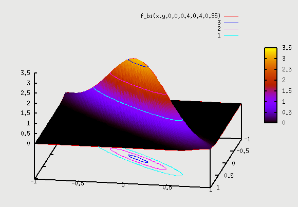
3. f(x,y) with ρ=0.95 =>Here correlation goes to extreme. We can consider the example of same people as above but Y axis as "score in Algebra2" and X axis as "score in Algebra1". We hope to see very strong correlation, as someone who scores well in Algebra1 will have high probability of scoring well in Algebra2. Similarly someone who scored bad in Algebra1 will have high probability of scoring bad in Algebra2 as well. The plot here starts becoming narrow ellipse and in the extreme case of ρ=1 becomes a 1D slanted copy of pdf of X. What that means is that Y doesn't even have a distribution given X. i.e if we are told that X=57 is the score, then Y is fixed to be Y=59 => Y doesn't have a distribution anymore given a particular X. In real life, Y will likely have a distribution for ex. from Y=54 to Y=60 (+3σ to -3σ range). This data is again going to come from field observation.


gnuplot> splot f_bi(x,y,0,0,0.4,0.4,0.95)


Let's see the example in detail once again for all values of ρ => If there are 5 kids with Algebra1 scores of (8,11,6,9,10) at -3σ, then if we go and look at Algebra2 score of these 5 kids, that will tell us the value of ρ. If scores in Algebra2 are all over the place from 0 to 100 (i.e 89, 9, 50, 75, 32) then we have no dependence and 2D contour plot looks like circle. However, if we see Algebra2 scores for these 5 kids are in narrow range as (7,10, 6,11,12), then this has a high dependence and the 2D contour plot looks like a narrow ellipse. This indicates a high value of ρ.

Also, we observe that as ρ goes from ρ=0 (plot 1) to ρ=1 (plot 3) the circle starts moving inwards, and squeezed into an ellipse. So points with some probablility for plot 1 (let's say 0.01 is combined pdf for point A on circle) have moved inwards for same probability for plot 2 and further in for plot 3. Also, the height of 3D plot goes up as the total pdf has to remain 1 for any curve. It's not too difficult to visualize this. Consider a (-3σ, -3σ) point for X and Y axis. This point has probability of 0.003*0.003 = 0.00001 for plot 1 where ρ=0 (i.e X and Y are independent). Now with  ρ=1 (plot 3), the -3σ point for X axis has probability of 0.003, but -3σ point for Y axis has probability of 1 (since with full correlation, Y has 100% probability of being at -3σ  when X is at -3σ). So, probability of (-3σ, -3σ) point is 0.003*1=0.003. So, this point now moves inward into the ellipse. The original point of 0.00001 probability is not (-3σ, -3σ)  point anymore. It looks like (-4σ, -4σ) point now lies closer to that original point, since it's probability is 10^-4*1=0.0001. Even this is higher. Maybe be more like (-4.5σ, -4.5σ) point lies on that point. So, we see how the correlation factor moves the σ points inwards.

2D plot for different samples:

In all the above plots we considered a sample of people and plotted different attributes of same sample of people. However, if we are plotting attributes of different samples, then it gets tricky. For ex, let's say we plot height of women vs height of men. What does it mean? Given pdf of height of men and pdf of height of women, what does combined pdf mean? Does it mean => given men of height=5ft with prob=0.1, and women of height 4ft with prob=0.2, what is the combined probability of finding men of height=5ft AND women of height=4ft. Best we can say is that are independent and so combined prob=0.1*0.2=0.02. So, we expect to see plot which is going to be similar plot as 1 above (with ρ=0). But how do we get field data for this sample to draw a 2D plot. Do we choose a man, and then choose a woman? The combined 2D pdf doesn't make sense, as men and women are 2 different samples.

However, we know that in a population where people are shorter, both men and women tend to be shorter, and in a population where people are taller, both men and women tend to be taller. So, if we take a sample of people, where men's height varied from 6ft to 7ft, and plotted women's height from that community, we might see that their height varies from 5.5ft to 6.5ft. Similarly for population where men's height varied from 5ft to 6ft, and plotted women's height from that community, we might see that their height varies from 4.5ft to 5.5ft. These are local variation within a subset, instead of global variation. If we take all of these local plots, and combine hem into a global plot, then we can get the dependence data. They suggest some correlation. If we plot all of these on our 2D plot, we may see that ρ≠0. We will see ellipse instead of a circle for iso contours of these 2D plot. These kind of plots are very common in semiconductors that we will see later.

Properties: A lot of cool properties of normal distribution appear, if we take the random variables to be independent, i.e ρ=0. Let's look at some of these properties:

Sum of independent Normal RV: Below is true ONLY for independent RV. If RV have ρ≠0, then below property is not true any more.

If X1, X2, ...Xn are independent normal random variables, with means \mu _{1}, \mu _{2} , ..and standard deviations \sigma _{1}, \sigma _{2}, ... then their sum X1+X2+...+xn will also be normally distribute with mean μ1 + μ2 + ...+ μn

and variance σ12 + σ22 + ... + σn2.

A proof exists here: https://online.stat.psu.edu/stat414/lesson/26/26.1


Probability & Statistics

These 2 go together. Probability is the basic foundation for statistics. It's basic knowledge is needed in a couple of things that we do in AI and in VLSI.

Basic probability:

https://en.wikipedia.org/wiki/Probability_theory

Probability is a number from 0 to 1 => 0 means 0% probability and 1 means 100% probability. Probability of an event is rep by letter "P" => P(event). Sum or integral of probability of all possible outcomes will always be 1.

Discrete Probability Distribution: This is for events that are countable, i.e throwing a dice, tossing coin, etc.

P(X) = 0.4 => Probability of event "X" happening is 40%.

If we roll a dice, then probability of any number 1 to 6 showing up is 1/6. P(dice=1)=1/6, P(dice=6)=1/6

Continuous Probability Distribution: This is for events that occur in continuous space, i.e temperature of water, etc.

PDF: Probability distribution function: When we have a function which is continuous, then instead of having discrete probability number, we have continuous probability function. This is called pdf. Integral of pdf over all possible outcomes will be 1 (just as in discrete case, the sum was 1)

P(x1<x<x2) = ∫ f(x)dx, where f(X) is the pdf, and integral is taken over limits x1 to x2

Factorial:

Factorial is defined as multiplication of all numbers less than or equal to that number. It's denoted by ! mark. So, 3!=3*2*1. 1!=1. n!=n*(n-1)...*2*1

n! = n*(n-1)!.

We define 0! as 1, as that keeps it consistent with other mathematical formulas used in Permutation and Combination shown below. It seems like 0! should be 0, but keeping it 1 allows it to blend nicely with Permutation formula for non-zero numbers.  We'll see that below.

Permutation and Combination:

The most important concept related to probability is figuring out all outcomes that are asked for a given event and divide it by all possible outcomes. As an ex, if probability of getting a 7 on throwing 2 dice is to be calculated, we can calculate as follows:

Number of ways 7 is possible E(sum=7)= (1,6), (2,5), (3,4), (4,3), (5,2) and (6,1) = 6 ways

Total number of possibilities of any number E(any sum) = 6 possibilities of 1st dice (1..6) * 6 possibilities of 2nd dice (1..6) = 6*6 = 36 ways

So, probability of getting 7 = E(sum=7)/E(sum=anything) = 6/36 = 1/6

Number of

Another general probability question is when we have to choose few things out of a given set of things, and we want to know of all different ways of doing it. This is where Permutation/Combination comes in. There are 2 handy formulas that we can use.

This link has very good explanation with the formula at the end: https://www.mathsisfun.com/combinatorics/combinations-permutations.html

  1. Permutation: Here order matters in arranging (P means Position, easy way to remember). ex is 4 digit gate lock code. It's a unique 4 digit code, so order of number matters (i.e 4756 is different than 4567).
    • Repetition not allowed: Given n things, if we have to choose r things, then total number of permutations possible = n*(n-1)*...*(n-r+1) = n!/(n-r)! where ! represents factorial. It's rep as nPr = n!/(n-r)!
      • ex: If we have to choose 3 balls out of 5 different colored balls, it can be done in 5*4*3=5!/2!=60. If we have to choose 1 ball, then it's 5!/4!=5 (as any colored ball can be chosen in every choice). If we have to choose 5 balls, then we can do it in 5*4*3*2*1=120 ways. So, 5!/(5-5)! = 5!/0!= 120 ways. The only way this could be 120 is if we choose 0! as 1. That's why we see in factorial section that 0!=1. If we have to choose 0 balls, then we can do it in 1 way. So, it's 5!/(5-0)! (as there's nothing to choose, so empty set is chosen which is just one way of choosing). So, 5!/5!=1
    • Repetition allowed: Given n things, if we have to choose r things, then total number of permutations possible = n^r
  2. Combination: Here order doesn't matter in arranging. ex is choose 3 socks out of a bag full of socks of different colors. The order in which you take the socks out doesn't matter, as we are concerned only about what color the socks are (i.e "red green blue" is no different than "blue green red").
    • Repetition not allowed: Given n things, if we have to choose r things, then we saw the total number of permutations possible in the above permutation case: It's nPr = n!/(n-r)!. We can easily see that for each set of "r distinct things", we have r! possible permutations. These all need to be grouped into one possibility, since we don't care about different permutations anymore. We are just interested in each such group of "r distinct things". So, we can divide the result by r! to get all combinations possible. So, number of combinations are = n!/((n-r)!*r!). It's rep as nCr = n!/((n-r)!.r!).
    • Repetition allowed: Given n things, if we have to choose r things where things can be repeated and order doesn't matter, then it's not as straight forward as the permutation case. An ex of this would be choosing 3 scoops from 5 flavors of ice cream, where each scoop can be any flavor. How many such combinations exist. One way to solve it would be divide it in 3 diff cases:
      • case 1: all 3 flavors are same => 5 such combinations possible.
      • case 2: 2 flavors are same. Here for each duplicated flavor, the remaining flavor can be one of 4 remaining ones, so 5 possibilities. But each dual flavor itself can be of 5 types, so total possibilities = 5*4=20
      • case 3: all 3 flavors are different. This is case of "repetition not allowed for combination" which is nCr = 5C3 = 5!/(3!*2!)=10
      • So, total number of combinations possible = 5+20+10=35
      • However, we can solve it other way, suggested in link above. We can put circle for each flavor selected and "x" for each time we move to next flavor. So, "x" serves to separate out diff flavors. In this ex, we 'll have exactly 3 circles and 4 "x". So, basically we are looking for all ways of arranging 3 circles in 7 positions.

Problems: Permutation + Combination

One of the biggest confusions in solving permutation/combination problems is to figure out whether the problem is a permutation problem or a combinatorial one. Many times it's not clear, and sometimes it's a mix of the 2. We'll look at some common problems below.

  1. Permutation of identical things: Let's say we have 2 balls, they may be identical or different. We have 5 slots arranged in a line, in which we need to put these balls, with only one ball going into 1 slot. How many ways can we arrange this?
    • 1st case: similar balls: Let's say the balls are of 2 colors = red and blue. First ball has 5 places to go, while 2nd ball has 4 places to go, so total places is 5*4=20 possibilities. This is simple permutation problem. The 3 slots remain empty, and there's no permutation possible amongst 3 empty slots, as empty slots are identical. Formula is nPr where we are placing r different things in n slots.
    • 2nd case: identical balls: Now let's say the 2 balls are identical. So, now we have to see in how many ways can this pair of 2 balls be arranged. The 1st ball can go in 5 places, just like before. 2nd ball can still go in 4 places, but many of the cases are now repeated, as balls are identical.
      • So, let's solve it other way as shown below.
        • Keeping 1st ball in position 1, we have 4 positions for ball 2. => Total ways = 4 ways
        • Keeping 1st ball in position 2, we have 3 positions for ball 2. => We can't put 2nd ball in position 1, as we already covered that case above. Total ways = 3 ways
        • Keeping 1st ball in position 3, we have 2 positions for ball 2. => We can't put 2nd ball in position 1 or position 2, as we already covered those cases above. Total ways = 2 ways
        • Keeping 1st ball in position 4, we have 1 position for ball 2. => On similar lines as above, other cases are already covered. Total ways = 1 way
        • Keeping 1st ball in position 5, we have no more unique places left for ball 2 to go. So Total = 0 ways.
        • So, In total, we get => 4+3+2+1 = 10 ways for the pair of 2 balls to go.
      • There's one other way to solve it. Since we are choosing 2 balls, and the order of balls doesn't matter (since they are identical), of all the 20 possibilities of permutation that we had with red and blue ball, we have to cut it down since red ad blue are same color now. So, this is a "combination" problem, where the order doesn't matter. So, we can divide 20 by 2! since 2! is the number of ways that this Red+blue balls were permutated amongst each other. So, total number of ways = 10. This way is lot easier to understand.
      • So, our formula for this permutation problem uses combinatorial part too.  In short, when having identical things r1, r2, ... rn, etc out of a total of r things, and having n slots, the formula is:
        • nPr / ((r1!)(r2!)...(rn!)) => We just took the permutation part and divide it by factorial of how many identical things we have in each set.


Basic Statistics:

https://en.wikipedia.org/wiki/Mathematical_statistics

Satistics is widely used in AI. There is a channel called "StatQuest" on Youtube that I found very helpful on learning basic statistics:

https://www.youtube.com/channel/UCtYLUTtgS3k1Fg4y5tAhLbw

For any sample X, where x1, x2, ..., xn are the individual samples in X, we define various terms that are very important in stats. Let's review these terms:

  • Mean(X) = 1/n * ∑ X  => Mean or average of any sample is sum of all values divided by number of sample points.
  • Variance(X) =  1/n * ∑ (X-Xmean) ^2 => variance is just measuring how far values are scattered from their mean value, on average. So, if X values are close to each other, Var(X) is small. Std deviation is just square root of Variance, i.e std_deviation(X) = σ(X) = √ Variance(X). So, variance(X) = σ2(X). Std deviation is more helpful in practical scenarios, since it represents variation from mean, and NOT the square of variation from mean.
  • Covariance(X,Y) = 1/n * ∑ ( (X-Xmean) * (Y-Ymean) ) => covariance measures joint variance of X and Y (Y is corresponding value for a given X for a set of n samples). Covariance is largest when X,Y move together, and is negative when they move opposite from each other. Covariance is 0, when there is no relation b/w X and Y (i.e X,Y are scattered all over the place). Covariance measures relationship b/w 2 different data, i.e are they related in some way or are they totally unrelated.


Central Limit Theorem (CLT):

It is one of the great results of mathematics. It's used both in Probability and statistics. IIt's not going to be used anywhere in our material, but it's good to know this. It establishes the importance of "Normal Distributiion". Theorem is stated in link below:

https://en.wikipedia.org/wiki/Central_limit_theorem


ETS:

ETS is encounter timing system, which is a STA timing tool from cadence. It's similar to PT.

Steps: Below are the steps to run ETS.


dir: /db/proj_ch/design1p0/HDL/ETS/digtop
cmd: ets -10.1_USR1_s096 -nowin -f scripts/check_timing_mmmc.tcl | tee logs/run_et_mmc_timing.log => -nowin means no window, else gui window comes up

File: scripts/check_timing_mmmc.tcl:
----
setDesignMode -process 250 => sets process tech to 250nm. For 180nm, use 180. For 150nm, use 150.

#read min/max lib
read_lib -max /db/../synopsys/src/PML30_W_150_1.65_CORE.lib /db/../synopsys/src/PML30_W_150_1.65_CTS.lib

read_lib -min /db/.../synopsys/src/PML30_S_-40_1.95_CORE.lib /db/.../synopsys/src/PML30_S_-40_1.95_CTS.lib

#read verilog
read_verilog ../../FinalFiles/digtop/digtop_final_route.v

set_top_module digtop => only when we run this, is when all max/min lib, netlist files are analyzed.

source scripts/create_views.tcl => source views file, same as from Autoroute dir

set_analysis_view -setup {func_max func_min scan_max scan_min} -hold {func_max func_min scan_max scan_min}

#set propagated clk by entering interactive mode
set_interactive_constraint_modes [all_constraint_modes -active]
set_propagated_clock [all_clocks]
set_clock_propagation propagated
set_interactive_constraint_modes {}

#read min/max qrc spef files
read_spef -rc_corner max_rc ../../FinalFiles/digtop/digtop_qrc_max_coupled.spef
read_spef -rc_corner min_rc ../../FinalFiles/digtop/digtop_qrc_min_coupled.spef

#wrt sdf
write_sdf -min_view func_min -max_view func_max -edges check_edge ./sdfs/digtop_func.sdf => has both min/max not in same file
write_sdf -min_view func_max -max_view func_max -edges check_edge ./sdfs/digtop_func_max.sdf => min/max are both equal to max
write_sdf -min_view func_min -max_view func_min -edges check_edge ./sdfs/digtop_func_min.sdf => min/max are both equal to min

NOTE: synopsys sdc file used in create_views.tcl is used to gen the delay in sdf file. set_load units may not get set appr, causing mismatch in delay num for all o/p buffers b/w SNPS sdf and CDNS sdf. Look in PnR_VDI.txt for more info.

#set_analysis_mode: sets analysis mode for timing analysis.
#-analysisType => single: based on one op cond from single lib, bcwc: uses max delay for all paths during setup checks and min delay for all paths during hold check from min/max lib, onChipVariation: for setup, uses max delay for data path, and min delay for clk path, while for hold, uses min delay for data path, and max delay for clk path. default is onChipVariation.
#-cprr < none | both | setup | hold > => removes pessimism from common portion of clock paths. none: disables removoal of cprr, while both enables cprr for both setup and hold modes. default is none.

set_analysis_mode -analysisType bcWc -cppr both

#setAnalysisMode => this is the equiv cmd in vdio as set_analysis_mode in ETS. diff is that default analysisType is set to single (if only 1 lib is provided) or bcwc (if 2 lib are provided).

#set_delay_cal_mode -engine aae -SIAware true => this is used to set timing engine, as well as to specify if we want SI(similar to PTSI)

#log file in log dir to report timing, clk, violations, etc. If this file is clean, no need to look at files in rpts dir.
check_timing -verbose >> $check_timing_log
report_analysis_coverage >> $check_timing_log
report_case_analysis >> $check_timing_log
report_clocks >> $check_timing_log
report_constraint -all_violators >> $check_timing_log => If we see any max_cap violation, we can run "report_net_parasitics -rc_corner " to find out cap of that net. We can get gate cap of all load atached from .liberty files. NOTE: wire/via cap(in rc table) and gate cap(in stdcell lib) changes with corners.
report_inactive_arcs >> $check_timing_log => This is put at end of file since it's very long.

# generate separate reports for setup and hold for func/scan
# report_timing: reports timing (used in vdio/ets)
#-early/-late => use -early for hold paths and -late for setup paths.
#-path_type full_clock => shows full expanded path (in PT, we use full_clock_expanded to get same effect)
#-max_paths => max # of worst paths irrespective of end points (i.e paths with same end points will show up multiple times here). If we do not want to see multiple paths with same end point, we can exclude those by using -max_points. In this case, it shows only 1 worst path to each end point. If we want to see specific # of paths to each end point, use -nworst option along with -max_points. We can only use one of the 2 options => max_paths or max_points.
#-net => adds a row for net arc. This separates net delay from cell delay (else by default: net delay is added to the next cell delay)
#-format { .. } => default format is: {instance arc cell delay arrival required}. With -net option, it shows net also. net delay is shown with i/p pins (A,B,C), while cell delay is shown for o/p pins (Y). additional options as load, pin_load, wire_load are also helpful.
#-view => By default, the command reports the worst end-point(s) across all views. if we want to view results for a particular view. use that view. The view should have already been created using "create_analysis_view" and set using "set_analysis_view". i.e:
=> create_analysis_view -name func_max -delay_corner max_delay_corner -constraint_mode functional
=> create_analysis_view -name func_min -delay_corner min_delay_corner -constraint_mode functional
=> set_analysis_view -setup {func_max func_min} -hold {func_max func_min} => now, we can run setup or hold analysis on both func_max and func_min. For this run, we already set view to "-setup {func_max func_min scan_max scan_min} -hold {func_max func_min scan_max scan_min}"
report_timing -from -to -path_type full_clock -view func_max -early => reports partcular hold path for view func_max. NOTE that this will work only if hold is calc for analysis_view "func_max".

#func setup/hold at func_min/func_max
#if we do not specify -view below, then all views set currently will be used. So, for "early" all views "func_max, func_min, scan_max, scan_min" will be used and shown in the single report. Each path will show a view so it's easy to see which view was used for that particular timing of path. However, it's better to separate out func view and scan view reports. We could have also set_analysis_view to just func_max/func_min for this run, and then for the 4 scan reports, we could have set views to just scan_max/scan_min. It's same either way.
report_timing -path_type full_clock -view func_max -max_paths 2000 -early -format {instance cell arc load slew delay arrival required} >> $func_rptfilename
report_timing -path_type full_clock -view func_max -max_paths 2000 -late -format {instance cell arc load slew delay arrival required} >> $func_rptfilename
report_timing -path_type full_clock -view func_min -max_paths 2000 -early -format {instance cell arc load slew delay arrival required} >> $func_rptfilename
report_timing -path_type full_clock -view func_min -max_paths 2000 -late -format {instance cell arc load slew delay arrival required} >> $func_rptfilename

#scan setup/hold at scan_min/scan_max
report_timing -path_type full_clock -view scan_max -max_paths 2000 -early -format {instance cell arc load slew delay arrival required} >> $scan_rptfilename
report_timing -path_type full_clock -view scan_max -max_paths 2000 -late -format {instance cell arc load slew delay arrival required} >> $scan_rptfilename
report_timing -path_type full_clock -view scan_min -max_paths 2000 -early -format {instance cell arc load slew delay arrival required} >> $scan_rptfilename
report_timing -path_type full_clock -view scan_min -max_paths 2000 -late -format {instance cell arc load slew delay arrival required} >> $scan_rptfilename

exit

---------
Timing reports in ETS:

ex: recovery check
Path 1842: MET Recovery Check with Pin Iregfile/tm_bank3_reg_6/C
Endpoint: Iregfile/tm_bank3_reg_6/CLRZ (^) checked with trailing edge of 'clk_latch_reg' => generated clk(div by 2 of osc_clk). so waveform is 1 101 201
Beginpoint: Iclk_rst_gen/n_reset_neg_sync_reg/Q (^) triggered by trailing edge of 'osc_clk' => created clk with waveform 1 51 101
Analysis View: func_max => shows view, doesn't show path group
Other End Arrival Time 104.067 => denotes capture clk timing
- Recovery 0.592 => recovery time for LAH1B from lib (+ve number in lib). +ve means it should setup sometime before the clk edge. So, we subtract recovery time from clk path delay. For setup, we subtract setup time, while for hold we add hold time.
+ Phase Shift 0.000 => This is the clock period for setup(for 10MHz clk, it's 100ns phase shift added for next clk edge)
+ CPPR Adjustment 0.000
= Required Time 103.475 => clk path delay
- Arrival Time 61.653 => data path delay
= Slack Time 41.822

=> start of data path (launch path)
Clock Fall Edge 51.000 => start point of clk fall
+ Drive Adjustment 0.041 => adjusted by driver for clk (invx1 or so), this number is added within clk/data path for PT, after the source latency number.
= Beginpoint Arrival Time 51.041
Timing Path: => data path as in PT
------------------------------------------------------------------------------------------------------------
Instance Cell Arc Load Slew Delay Arrival Required
Time Time
------------------------------------------------------------------------------------------------------------
clkosc v 3.312 0.064 51.041 92.863 => clk fall at 51.04ns
clkosc__L1_I0 CTB02B A v -> Y v 53.942 0.224 0.308 51.349 93.171 => clktree latency
clkosc__L2_I3 CTB45B A v -> Y v 62.517 0.346 0.488 51.837 93.659 => clktree latency
Iclk_rst/n_sync_reg DNC12 CLK v -> Q ^ 72.593 2.889 2.026 53.863 95.685
Iregfile/U171 NO211 A ^ -> Y ^ 55.505 4.133 2.999 56.862 98.684
Iregfile/FE_OFC0_n12 BU110J A ^ -> Y ^ 77.212 3.081 2.460 59.322 101.144
Iregfile/FE_OFC1_n12 BU110J A ^ -> Y ^ 72.938 2.919 2.235 61.557 103.379
Iregfile/tm_reg_6 LAH1B CLRZ ^ 72.938 2.927 0.096 61.653 103.475 => final arrival time of clrz
------------------------------------------------------------------------------------------------------------

=> start of clk path (capture path)
Clock Rise Edge 1.000 => start point of clk rise
+ Drive Adjustment 0.082
# + Source Insertion Delay -1.267 => insertion delay added if indicated in constraints (usually not present)
= Beginpoint Arrival Time 1.082 => final clk after adjusting for driver
Other End Path: => clk path as in PT
-----------------------------------------------------------------------------------------------------------------------------------
Instance Cell Arc Load Slew Delay Arrival Required Generated Clock
Time Time Adjustment
-----------------------------------------------------------------------------------------------------------------------------------
clkosc ^ 3.312 0.154 1.082 -40.740 => clk rise at 1.08ns
clkosc__L1_I0 CTB02B A ^ -> Y ^ 53.942 0.266 0.300 1.383 -40.440 => clktree latency
clkosc__L2_I4 CTB45B A ^ -> Y ^ 58.511 0.390 0.409 1.791 -40.031 => clktree latency
Ireg/wr_stb_sync_reg DTCD2 CLK ^ -> Q v 5.878 0.250 0.564 102.355 60.533 clk_latch_reg Adj. = 100.000 => falling edge of latch clk is setup edge for data. So, clk adjustment is done by 100ns (1/2 clk_latch_reg cycle). In PT, this adjustment is done in start of clk path.
Ireg/U176 AN2D0 B v -> Y v 46.242 1.848 1.702 104.057 62.235
Ireg/tm_bank3_reg_6 LAH1B C v 46.242 1.847 0.011 104.067 62.245
-----------------------------------------------------------------------------------------------------------------------------------

Ex: For SR latches, data to data checks done:
#Path 4: VIOLATED Data To Data Setup Check with Pin Imtr_b/itrip_latch_00/SZ => indicates SZ is clk
#Endpoint: Imtr_b/itrip_latch_00/RZ (^) checked with leading edge of 'clk_latch_reg' => indicates RZ is data (endpoint of data is RZ). clk_latch_reg refers to clk of SZ pin.
#Beginpoint: mtr_b_enbl (v) triggered by leading edge of 'osc_clk' => indicates startpoint of data is mtr_b_enbl pin. osc_clk refers to the clk firing the mtr_b_enbl signal. So, osc_clk is also the clk firing RZ, as there's only comb logic b/w mtr_b_enbl signal and RZ pin.
#Path Groups: {in2reg}
#Other End Arrival Time 1.861 => this is clk delay for SZ starting from created or generated clk. here, it's gen clk "clk_latch_reg".
#- Data Check Setup 0.036 => this is internal data setup req of latch wrt clk. here, RZ should come 0.036ns before SZ, so subtracted
#+ Phase Shift -100.000 => now, actual phases of clks taken into account (in PT, phase shifts are part of data/clk delays, but not in ETS). here, osc_clk has period of 100ns, while clk_latch_reg has period of 200ns. since SZ(clk) comes from clk_latch_reg, it may change at 0ns or 200ns or 400ns and so on, while RZ(data) coming from osc_clk may change at 0ns or 100ns or 200ns and so on. For data to data setup, we try to meet data setup wrt first clk edge. First SZ +ve edge is at 0ns, while worst case RZ +ve edge occurs at 100ns (if RZ +ve edge at 0ns chosen, then easy to meet timing, also if RZ +ve edge at 200ns chosen, then 2nd +ve edge of SZ would be chosen, which makes this pattern repeat, so we choose worst possible setup which is 100ns in this case). Phase shift is added to clk.
#= Required Time -98.175
#- Arrival Time 22.125 => this is data delay for RZ rising starting from mtr_b_enbl pin
#= Slack Time -120.299 => final slack

PrimePower (PP):

Synopsys PrimePower Product family analyzes power consumption of design at various stages starting from RTL all the way to final PnR netlist. PrimePower provides vector-free and vector-based peak power and averaged power analysis capabilities for RTL and gate-level designs. It calculates the power for a circuit at the cell level and reports the power consumption at the chip, block, and cell levels. Supported power analysis modes include average power, peak power, glitch power, clock network power, dynamic and leakage power, and multivoltage power;

There are 2 flavors of PrimePower:

  1. PrimePower RTL: This measures power consumption at RTL level. PrimePower RTL leverages the Predictive Engine from the RTL Architect tool and synthesis engine to synthesize RTL under the hood and analyze RTL for power.
  2. PrimePower (Gate level): When we say PrimePower only (without RTL), it means PrimePower for gate level power. During implementation and signoff, PrimePower provides accurate gate-level power analysis report based on actual netlist. 2 power analysis modes are supported for gate level - avg mode and time based mode.


Using PrimePower:

PrimePower may be used standalone, or may be invoked from within other Synopsys tool as PrimeTime. Also PT may be invoked from within PP. Both tools share many of the same libraries, databases, and commands, and support power and timing analysis. We need separate licenses of PrimePower and PrimeTime irrespective of which way they are invoked. These are the 2 ways:

  1. PWR_SHELL by Invoking PP: invoke PP by typing pwr_shell on the terminal. From within PP, we can invoke PT too.
    • pwr_shell> set power_enable_timing_analysis true => This invokes PT from within PP. Either we can read PT session from some other run, or generate timing data directly.
  2. PT_SHELL by Invoking PT: invoke PT by typing pt_shell on the terminal. Then PP may be invoked from within PT. This keeps timing and power numbers in one place and eliminates need for PP standalone setup.
    • pt_shell> set power_enable_analysis true => This invokes PP from within PT. Either we can read PP session from some other run, or generate Power data directly.

PrimePower (PP) and PrimeTime-PX (PT-PX):

When Synopsys initially came with their Power tool in 2000's, it used the 2nd option above (i.e Power tool was invoked from within PT). They called this tool PT-PX or PT with Power Analysis. Even though it was invoked from within PT_SHELL, it required separate license of PT-PX  to run power. This tool calculated power only at gate level. Later they added the capability to calculate power at RTL level. This required power tool to be invoked separately. So, they introduced PrimePower (PP) as a standalone tool for Power analysis. PP could be invoked for both RTL and gate level Power. PT-PX was rebranded as belonging to "PrimePower family". Synopsys confirmed that PP is actually a superset of PT-PX, so PP should be used going forward (Do NOT use PT-PX anymore as of 2025). For our purpose, PT-PX is treated same as PP in notes below (as the notes are from 2023, when I was still using PT-PX). 

Startup File: When PP or PTPX is invoked, we can have an optional synopsys startup file that will be sourced on startup. It's similar to PT startup file:.synopsys_pt.setup

PP/PT-PX combines simulation time window to report power within a window. All the options and cmds are almost same for PP and PT-PX. Inputs and Outputs are same too.

Inputs:

  • Library: A cell library containing timing and pwr characterization info for each cell.
  • Gate level netlist: In verilog, VHDL or Synopsys db format.
  • Design constraints: An SDC file containing design constraints to calculate the transition time on the primary inputs and to define the clocks.
  • Switching activity: The design switching activity information which can be specified in an event file in the VCD or FSDB format.
  • Net parasitics: A parasitics file (SPEF) containing net capacitances for all the nets.

Outputs

  • Various power reports.

 2 Imp terms in Power:

  • Static probability (SP) => This is the probabilty of a signal to be at logic 0 (SP0) or logic 1 (SP1). If SP1=0.7, it implies that the signal is at logic 1 for 70% of the time. By default, SP0 and SP1 are 0.5, implying logic is 1 for one half the time.
  • Toggle rate (TR) => This is the number of 0-to-1 and 1-to-0 logic transitions of a design object per unit of time, such as a net, a pin, or a port.
  • Switching activity => This consists of both the SP and TR.


PP:

PP can be invoked for both RTL and Gate. When we say PP, we mean gate level power runs. Only when we say PP-RTL is when we refer to PP running on RTL.

Steps:

Following are the steps to invoke PP:

0. Invoke pwr_shell normally => As you would for PT timing runs

pwr_shell -2012.12-SP3 -f scripts/run_power.tcl | tee logs/run_power.log => run_pwer.tcl has cmds for running power flow, so that we can run in batch mode (i.e automated). If we don't want it automated we can type the cmds on pt_shell too. By default, all cmds processed by tool including those in setup file are dumped in pwr_shell_command.log. PP can be invoked in gui mode too by using -gui option (pwr_shell -gui). In gui mode, it's easy to enter further cmds as it's just selecting required items from menu list. 

GUI: To start gu from within shell (if not invoked at startup), type "gui_start" from pwr_shell window.

1. PT run: set library, read gate level verilog netlist and spef file => same as in normal PT flow. pwr is calc for chosen PVT corner.

### I. Below cmds are for regular PT runs
set search_path "$search_path /db/pdkoa/1533e035/current/diglib/pml48h/synopsys/bin"
set target_library PML48H_W_85_3_CORE.db
set link_library {* PML48H_W_85_3_CORE.db}

set_operating_conditions ...

read_verilog /db/MYCHIP/.../FinalFiles/digtop_final_route.v => read final routed netlist

load_upf /.../digtop_final.upf => if UPF is available
current_design digtop
link_design

read_parasitics /db/MYCHIP/.../FinalFiles/digtop_final_route_max.spef => read max spef file (this has parasitics, i.e R,C for all nets)

read_sdc /../digtop.sdc => has all constraints as clk defn, False paths, etc. This is needed for PT runs (not for PP)

#update_timing

check_timing

report_timing

2. PP run: set power analysis so that PTPX license is invoked

### II. Below cmds are for PP/PTPX runs

set power_enable_analysis true => This is what invokes PP from within PT.
set power_analysis_mode averaged | time_based

#set_power_derate => This can be sued to set derating factor for power rails or on specific cells, where the power is adjusted by a factor when calculating it. This allows us to adjust power as needed to match silicon power more closely (similar to how we use derating for timing).

check_activity

3. Read VCD or FSDB file from one of the simulation (it needs to be gate level VCD file with back annotation of parasitics)
read_vcd /sim/MYCHIP/.../sim1_max.vcd.gz -strip_path digtop_tb/IDUT/spi_regs -time {100489 800552} => strips module of interest so that pwr is reported starting from that module as top level. time is in ns.
#report_switching_activity > reports/power_swtching.rpt => to examine tr/sp (see below) and vcd file syntax

#write_activity_waveforms => generates activity waveforms from the activity file.

4. report power
#check_power -verbose => prior to analysis, verifies that analysis i/p are valid
#update_power => This is needed for RTL VCD or when no vcd provided to propagate activity to nets/registers not annotated from RTL VCD file.
#report_switching_activity => to examine propagated values of tr/sp
#create_power_waveforms -cycle_accurate => to show pwr waveform
report_power > ./reports/power_summary.rpt
report_power -hier > ./reports/power_hierarchy.rpt
#report_power -cell -flat -net -hier -verbose -nosplit > power_detail.rpt


save_session =>
exit


### 2. Now we start the powr runs (PP)

set_app_var power_limit_extrapolation_range true => By default, PP extrapolates indefinitely if the data point for internal power lookup is out of range (default value is FALSE). When set to TRUE, the tool limits the extrapolation. That is needed for more accurate pwr values when there are many high fanout nets as clks, reset in design.


2. Invoke PT or restore PT session


restore_session

check_power


PT-PX:

This is the flow when we want to invoke PT, and then from within PT, we invoke PT-PX.

Steps:

Following are the steps to invoke PT-PX:

0. Invoke pt_shell normally => As you would for PT timing runs

pt_shell -2012.12-SP3 -f scripts/run_power.tcl |tee logs/run_power.log => can be invoked in gui mode too. run_pwer.tcl has cmds for running power flow, so that we can run in batch mode (i.e automated). If we don't want it automated we can type the cmds on pt_shell too.

run_power.tcl script above has following cmds:


1. set library, read gate level verilog netlist and spef file => same as in normal PT flow. pwr is calc for chosen PVT corner.
set search_path "$search_path /db/pdkoa/1533e035/current/diglib/pml48h/synopsys/bin"
set target_library PML48H_W_85_3_CORE.db
set link_library {* PML48H_W_85_3_CORE.db}

read_verilog /db/ATAGO/.../FinalFiles/digtop_final_route.v => read final routed netlist
current_design digtop
link

read_parasitics /db/ATAGO/.../FinalFiles/digtop_final_route_max.spef => read max spef file

2. set power analysis so that PP license is invoked
set_app_var power_enable_analysis true => This is what enables Power Analysis from within PT. This cmd is needed, else PT-PX won't run.
set power_analysis_mode averaged

3. Read VCD file from one of the simulation (it needs to be gate level VCD file with back annotation of parasitics)
read_vcd /sim/ATAGO/.../sim1_max.vcd.gz -strip_path digtop_tb/IDUT/spi_regs -time {100489 800552} => strips module of interest so that pwr is reported starting from that module as top level. time is in ns.
#report_switching_activity > reports/power_swtching.rpt => to examine tr/sp (see below) and vcd file syntax

4. report power
#check_power -verbose => prior to analysis, verifies that analysis i/p are valid
#update_power => This is needed for RTL VCD or when no vcd provided to propagate activity to nets/registers not annotated from RTL VCD file.
#report_switching_activity => to examine propagated values of tr/sp
#create_power_waveforms -cycle_accurate => to show pwr waveform
report_power > ./reports/power_summary.rpt
report_power -hier > ./reports/power_hierarchy.rpt
#report_power -cell -flat -net -hier -verbose -nosplit > power_detail.rpt
exit


Restoring pt_shell:

We sometimes want to restore pt_Shell/pp_shell to do some debug work or to get more data on specific parts of design. We can restore pt_shell and then run below cmds:

pt_shell> report_power -cell_power [get_cells top/i_and2] => reports pwr components for given cell

                       Internal  Switching Leakage   Total
Cell                    Power     Power     Power     Power    (     %)   Attrs
--------------------------------------------------------------------------------
top/i_and2        0.0020    0.0300 1.426e-10 0.032 (100.00%)
--------------------------------------------------------------------------------
Totals (1 cell)    0.0020    0.0300 1.426e-10 0.032 (100.0%)

If we are writing a script to gather these numbers, then we can use "get_att" cmd to get pwr attr
pt_shell> list_attributes -application -class cell -nosplit => This lists all attr for cells. We see *power* attr

pt_shell> get_att [get_cells top/i_and2] internal_power => gives internal power. Similarly for switching_power, leakage_power and total_power. Also gives other pwr as dynamic_power, glitch_power, peak_power, etc.


Report: power summary report:

1. static power: Cell Leakage power. It's leakage in the cell from VDD to VSS when cell i/p is at 0 or 1 (subthreshold lkg from src to drn since gates never turn off completely). It includes gate lkg also (gate lkg is captured only for i/p pins for each transistor, as o/p pin will finally connect to i/p pin of some other transistor. gate lkg is just the current flowing into the gate when i/p of gate is 0 or 1). cell lkg pwr number comes from *.lib file. Pwr(lkg)=V*I(subthreshold_lkg)+V*I(gate_lkg).
It has a default lkg pwr number for each cell, as well as different lkg pwr numbers depending on diff i/p values. ex:
cell (AN210_3V) {
cell_leakage_power : 1.731915E+00; => default lkg pwr
leakage_power () { => we can have many of these conditions for each cell
value : 1.718650E+00; => lkg pwr = 1.7pW when A=1 and B=0. pwr unit defined as pw by "leakage_power_unit : "1pW";" in .lib file
when : "A&!B";
}

2. dynamic power: 2 components to this:


A. internal pwr: This includes short ckt pwr when cell o/p is switching, as well as pwr due to charging/discharging of internal nodes in the cell (due to src/drn cap on all o/p nodes and gate cap on internal nodes). cell int pwr number comes from *.lib file. Pwr(int)=Eint*Tr where Tr=number of toggles/time.
Just like timing() section, we have internal_power() section for o/p pin. It shows int pwr for each combination of i/p values slew rate and o/p cap load (as pwr will change due to short ckt current, drn/src cap changing). ex:

cell (AN210_3V) {
pin (Y) { => pwr is always for o/p pin, since i/p pin pwr is calculated separately as switching pwr.
internal_power () { => pwr unit is in pJ = power unit(pW) * time_unit(s) (it's energy, not power).
related_pin : "A"; => this is when o/p changes due to i/p pin A changing
rise_power (outputpower_cap4_trans5) { ... 34.39 .. } => pwr under diff cap load on o/p pin, and diff slew on i/p pin
fall_power (outputpower_cap4_trans5) { ... 34.39 .. } => fall_power is when o/p pin falls due to pin A rising/falling
}
internal_power () {
related_pin : "B"; => this is when o/p changes due to i/p pin B changing
rise_power (outputpower_cap4_trans5) { ... 34.39 .. } => rise_power is when o/p pin rises due to pin B rising/falling
fall_power (outputpower_cap4_trans5) { ... 40 .. } => 40pJ energy per toggle. Since time is in ns, pwr=mw??
}
}
}

B. switching pwr: This is due to charging/discharging of all the o/p load in design. This includes wire cap and gate cap on i/p pins which switch whenever o/p pin of any gate switches. Pwr(sw)=0.5*C*V^2*Tr. Tr=number of toggles/time.

Total_pwr = Pwr(lkg) + Pwr(int) + Pwr(sw) = Pwr(lkg) + Eint*Tr + 0.5*C*V^2*Tr (Pwr(lkg) and Eint come from.lib).
To calc avg pwr, static probability (Sp) is calcualted for all the nodes to be at 1 or 0. This is then used to calc lkg pwr for each cell. Toggle rate is caluclated for each node to calc dynamic pwr.
To calc peak pwr, vcd file is required to analyze events. It's useful for dynamic IR drop. If vcd file not provided, then tool doesn't know the seq of events. Merely toggle rate doesn't tell it whether all nodes toggle at same time or not.
When VCd file is not provided, default Tr/Sp is applied to starting points (PI, black box o/p). default Tr/Sp can be modified using (power_default_toggle_rate, power_default_static_probability)


PT-SI:

PT-SI is PT with Signal Integrity. PT-SI is basically  timing tool with crosstalk (requires separate license of PT-SI, regular PT license won't work)

link for discussion of si_xtalk_delay_analysis_mode option in PT-SI:
https://solvnet.synopsys.com/retrieve/015943.html?otSearchResultSrc=advSearch&otSearchResultNumber=4&otPageNum=1

PT-SI runs thru these steps:
1. electrical filtering, where aggressor nets whose effects are too small to be significant, based on the calculated sizes of bump voltages on the victim nets re removed. You can specify the threshold level that determines which aggressor nets are filtered. If the bump height contribution of an aggressor on its victim net is very small (less than 0.00001 of the victim’s nominal voltage), this aggressor is automatically filtered.
2. After filtering, PT SI selects the initial set of nets to be analyzed for crosstalk effects from those not already eliminated by filtering. You can optionally specify that certain nets be included in, or excluded from, this initial selection set.
3. The next step is to perform delay calculation, taking into account the crosstalk effects on the selected nets. This step is just like ordinary timing analysis, but with the addition of crosstalk considerations. This step runs in 2 iterations:
I. For the initial delay calculation (using the initial set of selected nets), PrimeTime SI uses a conservative model that does not consider timing windows.
II. In the second and subsequent delay calculation iterations, PT SI considers timing windows, and removes from consideration any crosstalk delays that can never occur, based on the separation in time between the aggressor and victim transitions or the direction of the aggressor transition. The result is a more accurate, less pessimistic analysis of worst-case effects. By default only 2 iterations done, as these provide good results. This variable is used to set no. of iterations. si_xtalk_exit_on_max_iteration_count => default to 2

logical correlation for buffers and inverters is considered in PTSI. For ex, if there is an inverter and both i/p and o/p nets of buffer are aggressing to a net, than these switch in opposite dirn, cancelling the x coupling effect, and resulting in very small delta delay or noise effect.

PT-SI is same as normal flow, except that we have to enable SI. These are the steps:
1. set target lib, link lib same way. set op cond to ocv.
2. Enable PT-SI (if we want to run SI)
set si_enable_analysis TRUE

3. set parameter for xtalk analysis
#For xtalk, default is to calc max delta delay for all paths (all_paths).
#set si_xtalk_delay_analysis_mode
#all_paths -> Calculate Max delta delay for all path through victim net. Could be pessimistic for critical paths for 2 reasons: Firstly, switching region of the victim is derived from the early and late timing windows without considering the individual subwindows that constitute it. Therefore, this might include regions where there is no switching on the victim. Second, the entire on-chip variation of the path is considered, creating the effect of multiple paths even when only a single path exists, for example, in a chain of inverters.
#all_path_edges -> considers only the edges of transition on victim net. This eliminates false overlap due to timing window caused due to multiple paths, and results in more accurate xtalk delay.
# worst_path -> DEPRECATED. do not use. Calculate Max delta delay only for critical path through victim. Accurate for critical path but could be optimisitic for non-critical paths. We pick victim critical path, so victim window is discrete edge, and false overlap of timing window is eliminated.
# violating_path -> DEPRECATED. do not use. Calculate Max delta delay for worst path and all <0 slack paths (recommended)
set si_xtalk_delay_analysis_mode all_path_edges

4. read verilog and parasitics as normal.
read_verilog /db/DAYSTAR/NIGHTWALKER/design1p0/HDL/FinalFiles/digtop/digtop_final_route.v
current_design $TOP
link

read_parasitics -keep_capacitive_coupling -format spef /db/DAYSTAR/NIGHTWALKER/design1p0/HDL/FinalFiles/digtop/digtop_qrc_max_coupled.spef => -keep_capacitive_coupling is needed to preserve all coupling cap from spef file. else, they will be grounded, and we wont see any noise effect. NOTE: spef file used here should have been generated with coupling caps in it (they should not be grounded). In EDI, it's done by generating spef after doing "setExtractRCMode -coupled true".
report_annotated_parasitics -check => make sure that coupling cap is shown here

5. read sdc constraints, check_timing, and then report timing for setup/hold.
report_timing -crosstalk_delta -delay max|min -path full_clock_expanded -nets -capacitance -transition_time -max_paths 500 -slack_lesser 2.0 => reports delta delay due to noise in GBA (can use -cross also instead of -crosstalk_delta). dtrans col in report shows delta transition caused due to xtalk, while delta col shows delta delay caused.
report_timing -crosstalk_delta -pba_mode exhaustive -delay max|min -path full_clock_expanded -nets -capacitance -transition_time -nworst 1 -max_paths 50 -slack_lesser 0.2 => reports delta delay due to noise in PBA.

PBA mode improves noise delay significantly because of 3 reasons: (https://solvnet.synopsys.com/retrieve/012134.html?otSearchResultSrc=advSearch&otSearchResultNumber=6&otPageNum=1)
A. slew rate is improved.
B. only single victim edge is considered for a single path of victim. Aggressor still have windows, as they can have multiple paths, but this reduces the overlap b/w victim and aggressor, resulting in elimination of lot of false victim window.
C. CPRR is improved, resulting in hold time improvement.

NOTE: PBA can't be used in sdf, as sdf has single delay value associated with each cell (it's a graph based rep).

6. static noise analysis: noise related reports. It uses noise modling from .lib or estimates noise based on delays/slew.
PTSI uses the following order of precedence when choosing which noise immunity information to use:
1.Static noise immunity curve annotated using the set_noise_immunity_curve command
2.DC noise margin annotated using the set_noise_margin command
3.Arc-specific noise immunity curve from library
4.Pin-specific noise immunity curve from library
5.CCS noise model from library
6.DC noise margin from library

#bottleneck for xtalk delta delay
report_si_bottleneck -cost_type delta_delay -significant_digits 3 => determine the major victim nets or aggressor nets that are causing multiple violations. reports the nets having the highest “cost function”. Four different cost functions:
1. delta_delay – Lists the victim nets having the largest absolute delta delay, among all victim nets with less than a specified slack.
2. delta_delay_ratio – Lists the victim nets having the largest delta delay relative to stage delay, among all victim nets with less than a specified slack.
3. total_victim_delay_bump – Lists the victim nets having the largest sum of all unfiltered bump heights (as determined by the net attribute si_xtalk_bumps), irrespective of delta delay, among all victim nets with less than a specified slack.
4. delay_bump_per_aggressor – Lists the aggressor nets that cause crosstalk delay bumps on victim nets, listed in order according to the sum of all crosstalk delay bumps induced on affected victim nets, counting only those victim nets having less than a specified slack.
By default, the specified slack level is zero, which means that costs are associated with timing violations only. If there are no violations, there are no costs and the command does not return any nets.

#nets reported by the bottleneck cmd are investigated with this cmd.
report_delay_calcualtion -crosstalk -from -to => provides detailed information about crosstalk calculations for a particular victim net. It shows active aggressors, reason for inactive aggressor, delta delay/slew and victim analysis.
I - aggressor has Infinite arrival with respect to the victim
N - aggressor does not overlap for the worst case alignment

#update_timing => updates timing due to xtalk, after "what if" fixes are made using size_cell and set_coupling_separation.
#update_noise => detects functional errors resulting from the effects of crosstalk on steady-state nets.

report_si_double_switching => determine those victim nets with double-switch violations in the design. Double-switching errors such can cause incorrect circuit operation by false clocking on the inactive edge of a clock signal, by double clocking on the active edge of a clock signal, or glitch propagation through combinational logic.

#static noise analysis:
#set_noise_parameters -ignore_arrival -include_beyond_rails -enable_propagation -analysis_mode report_at_source | report_at_endpoint
#-ignore_arrival => causes the arrival window information of the aggressors to be ignored during the noise analysis. Therefore, the aggressors are assumed to be always overlapping to maximize the effect of coupled noise bump.
#-include_beyond_rails => By default, the analysis of noise above the high rail and below the low rail is disabled. This option, enables the analysis of noise beyond the high and low regions.
#-enable_propagation => Specifies whether or not to allow noise propagation. Propagated noise on a victim net is caused by noise at an input of the cell that is driving the victim net. PrimeTime SI can calculate propagated noise at a cell output, given the propagation characteristics of the cell, the noise bump at the cell input, and the load on the cell output.
#-analysis_mode report_at_source | report_at_endpoint => In report_at_source mode, viol are reported at the source of violations. In report_at_endpoint mode, violations are propagated through fanout and reported at endpoints. default value is report_at_source.

NOTE: no noise models needed, as default is "report_at_source" mode, where noise bumps are not propagated, but rather fixed at source. controlled by "set_noise_parameters".
set_noise_parameters -enable_propagation => noise propagated.

#set_noise_margin, set_noise_immunity_curve => Specifies the bump-height noise margins or 3 coefficient values for an input port of the design or an input pin of a library cell, that determine whether a noise bump of a given height at a cell input causes a logical failure at the cell output. noise immunity of cell is provided here.

#set_si_noise_analysis => Includes or excludes specified nets for crosstalk noise analysis.

check_noise => checks the design for the presence and validity of noise models at driver and load pins. No pins should be found w/o noise constraints i.e. The number of pins reported in the “none” row of the report must be zero.

update_noise => performs a noise analysis and updates the design with noise bump information using the aggressor timing windows previously determined by timing analysis.
report_noise -all_violators => generates a report on worst-case noise effects, including width, height, and noise slack. It also determine those victim nets with double-switch violations in the design. -all_violators reports only those pins/nets that have -ve noise slack (i.e noise bump is above noise threhold). To get more detailed report, use -verbose.

#report_noise_calculation => generates a detailed report on the calculation of the noise bump on a net arc (single net). same as report_delay_calculation except that it reports noise instead of delay. The startpoint is the driver pin or driver port of a victim net and the endpoint is a load pin or load port on the same net.

7. inlcuding/excluding certain nets: (if you still have failures), and run delay/noise analysis again.
#set_si_delay_analysis – Includes or excludes specified nets for crosstalk delay analysis.
#set_si_noise_analysis – Includes or excludes specified nets for crosstalk noise analysis.
#set_si_aggressor_exclusion – Excludes aggressor-to-aggressor nets that switch in the same direction. Only specified number of aggressors (default 1) is active at a time.
#set_coupling_separation – Excludes nets or net pairs from crosstalk delay and crosstalk noise analysis.